Pauli correlation encoding to reduce max-cut requirements

Usage estimate: 35 minutes on an Eagle r3 processor (NOTE: This is an estimate only. Your runtime might vary.)

Learning outcomes

After going through this tutorial, users should expect the following outcomes:

Understand the theoretical principles behind Pauli Correlation Encoding (PCE), including how multi‑body Pauli strings enable polynomial compression of classical optimization problems.
Implement PCE in practice to encode and solve large‑scale optimization tasks on near‑term quantum hardware.

Prerequisites

We recommend familiarity with the following topics before going through this tutorial:

Background

This tutorial presents Pauli Correlation Encoding (PCE) [1], an approach designed to encode optimization problems into qubits with greater efficiency for quantum computation. PCE maps classical variables in optimization problems to multi-body Pauli-matrix correlations, resulting in a polynomial compression of the problem's space requirements. By employing PCE, the number of qubits needed for encoding is reduced, making it particularly advantageous for near-term quantum devices with limited qubit resources. Furthermore, it is analytically demonstrated that PCE inherently mitigates barren plateaus, offering super-polynomial resilience against this phenomenon. This built-in feature enables unprecedented performance in quantum optimization solvers.

Overview

The PCE approach consists of three main steps, as illustrated in Figure 1 from [1] in below:

Encoding the optimization problem into a Pauli correlation space.
Solving the problem using a quantum-classical optimization solver.
Decoding the solution back to the original optimization space. The PCE approach is adaptable to any quantum optimization solver capable of processing Pauli correlation matrices. 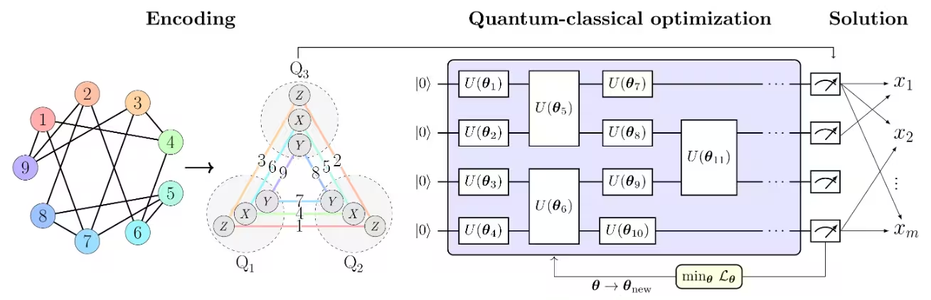In Figure 1 from [1], the max-cut problem is used as an example to illustrate the PCE approach. The max-cut problem with $m=9$ nodes is encoded into a Pauli correlation space, representing the optimization problem as a correlation matrix — specifically, two-body Pauli-matrix correlations across $n=3$ qubits $(Q_1, Q_2, Q_3)$ . Node colors indicate the Pauli string used for each encoded node. For example, node 1, which corresponds to binary variable $x_1$ , is encoded by the expectation value of $Z_1 \otimes Z_2 \otimes I_3$ , while $x_8$ is encoded by $I_1 \otimes Y_2 \otimes Y_3$ . This corresponds to compressing the problem's $m$ variables into $n = O(m^{1/2})$ qubits. More broadly, $k$ -body correlations enable polynomial compressions of order $k$ , with $k>1$ . The chosen Pauli set comprises three subsets of mutually-commuting Pauli strings, allowing all $m$ correlations to be experimentally estimated with only three measurement settings.

A loss function $\mathcal{L}$ of Pauli expectation values that imitates the original max-cut objective function is constructed. The loss function is then optimized using a quantum-classical optimization solver, such as the Variational Quantum Eigensolver (VQE).

Once the optimization is complete, the solution is decoded back to the original optimization space, yielding the optimal max-cut solution.

Requirements

Before starting this tutorial, be sure you have the following installed:

Qiskit SDK v1.0 or later, with visualization support
Qiskit Runtime v0.22 or later (pip install qiskit-ibm-runtime)

Setup

# Added by doQumentation — required packages for this notebook
!pip install -q networkx numpy qiskit qiskit-aer qiskit-ibm-runtime rustworkx scipy

from itertools import combinations

import numpy as np
import rustworkx as rx
import networkx as nx

from scipy.optimize import minimize, OptimizeResult

from qiskit.circuit.library import efficient_su2
from qiskit.transpiler.preset_passmanagers import generate_preset_pass_manager
from qiskit.quantum_info import SparsePauliOp
from qiskit_ibm_runtime import EstimatorV2 as Estimator
from qiskit_ibm_runtime import QiskitRuntimeService
from qiskit_ibm_runtime import Session
from rustworkx.visualization import mpl_draw
from qiskit_aer import AerSimulator

def calc_cut_size(graph, partition0, partition1):
    """Calculate the cut size of the given partitions of the graph."""

    cut_size = 0
    for edge0, edge1 in graph.edge_list():
        if edge0 in partition0 and edge1 in partition1:
            cut_size += 1
        elif edge0 in partition1 and edge1 in partition0:
            cut_size += 1
    return cut_size

Small-scale simulator example

service = QiskitRuntimeService()
real_backend = service.least_busy(
    operational=True, simulator=False, min_num_qubits=156
)
backend = AerSimulator.from_backend(real_backend)
print(f"We are using the {backend.name}")

We are using the aer_simulator_from(ibm_pittsburgh)

Step 1: Map classical inputs to a quantum problem

The max-cut problem

The max-cut problem is a combinatorial optimization problem that is defined on a graph $G = (V, E)$ , where $V$ is the set of vertices and $E$ is the set of edges. The goal is to partition the vertices into two sets, $S$ and $V \setminus S$ , such that the number of edges between the two sets is maximized. For the detailed description of the max-cut problem, please refer to the Quantum approximate optimization algorithm tutorial. The max-cut problem is also used as an example in the Advanced techniques for QAOA tutorial. In those tutorials, the QAOA algorithm is used to solve the max-cut problem.

Graph -> Hamiltonian

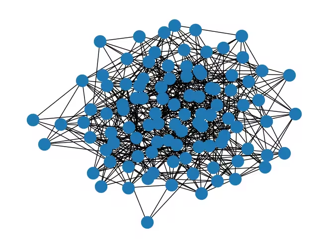
Let us first consider a random graph with 100 nodes.

num_nodes = 100  # Number of nodes in graph
seed = 42
graph = rx.undirected_gnp_random_graph(num_nodes, 0.1, seed=seed)
mpl_draw(graph)

Output of the previous code cell

nx_graph = nx.Graph()
nx_graph.add_nodes_from(range(num_nodes))

for edge in graph.edge_list():
    nx_graph.add_edge(edge[0], edge[1])

curr_cut_size, partition = nx.approximation.one_exchange(nx_graph, seed=1)
print(f"Initial cut size: {curr_cut_size}")

Initial cut size: 345

We encode the graph with 100 nodes into two-body Pauli-matrix correlations across nine qubits (see the explanation below). The graph is represented as a correlation matrix, where each node is encoded by a Pauli string. The sign of the expectation value of the Pauli string indicates the partition of the node. For example, node 0 is encoded by a Pauli string, $\prod_0 = I_{8} \otimes ... I_2 \otimes X_1 \otimes X_0$ . The sign of the expectation value of this Pauli string indicates the partition of node 0. We define a Pauli-correlation encoding (PCE) relative to $\prod$ as

$x_i \coloneqq \textit{sgn}(\langle\prod_i \rangle),$

where $x_i$ is the partition of node $i$ and $\langle \prod_i \rangle \coloneqq \langle \psi |\prod_i| \psi \rangle$ is the expectation value of the Pauli string encoding node $i$ over a quantum state $|\psi \rangle$ . Now, let's encode the graph into a Hamiltonian using PCE. We divide the nodes into three sets: $S_1$ , $S_2$ , and $S_3$ . Then, we encode the nodes in each set using the Pauli strings with $X$ , $Y$ , and $Z$ , respectively. We need to extract a relationship between the number of nodes and qubits that we will need to encode all the nodes. Using all possible permutations for the encoding yields to:

m=3\binom{n}{k}.

In this example we consider $k=2$ , hence,

m = \frac{3}{2} n(n-1).

Therefore, the number of qubits $n$ needed to express a certain number of nodes $m$ read as:

n = \left\lceil \frac{1 + \sqrt{1 + \tfrac{8}{3}m}}{2} \right\rceil.

Note that the $\lceil \cdot \rceil$ symbol represents the ceiling function, which rounds any real number up to the next integer. This ensures that the number of qubits is an integer.

num_qubits = int(np.ceil((1 + np.sqrt(1 + (8 / 3) * num_nodes)) / 2))

list_size = num_nodes // 3
node_x = [i for i in range(list_size)]
node_y = [i for i in range(list_size, 2 * list_size)]
node_z = [i for i in range(2 * list_size, num_nodes)]

print(f"Number of qubits: {num_qubits}")
print("List 1:", node_x)
print("List 2:", node_y)
print("List 3:", node_z)

Number of qubits: 9
List 1: [0, 1, 2, 3, 4, 5, 6, 7, 8, 9, 10, 11, 12, 13, 14, 15, 16, 17, 18, 19, 20, 21, 22, 23, 24, 25, 26, 27, 28, 29, 30, 31, 32]
List 2: [33, 34, 35, 36, 37, 38, 39, 40, 41, 42, 43, 44, 45, 46, 47, 48, 49, 50, 51, 52, 53, 54, 55, 56, 57, 58, 59, 60, 61, 62, 63, 64, 65]
List 3: [66, 67, 68, 69, 70, 71, 72, 73, 74, 75, 76, 77, 78, 79, 80, 81, 82, 83, 84, 85, 86, 87, 88, 89, 90, 91, 92, 93, 94, 95, 96, 97, 98, 99]

def build_pauli_correlation_encoding(pauli, node_list, n, k=2):
    pauli_correlation_encoding = []
    for idx, c in enumerate(combinations(range(n), k)):
        if idx >= len(node_list):
            break
        paulis = ["I"] * n
        paulis[c[0]], paulis[c[1]] = pauli, pauli
        pauli_correlation_encoding.append(("".join(paulis)[::-1], 1))

    hamiltonian = []
    for pauli, weight in pauli_correlation_encoding:
        hamiltonian.append(SparsePauliOp.from_list([(pauli, weight)]))

    return hamiltonian

pauli_correlation_encoding_x = build_pauli_correlation_encoding(
    "X", node_x, num_qubits
)
pauli_correlation_encoding_y = build_pauli_correlation_encoding(
    "Y", node_y, num_qubits
)
pauli_correlation_encoding_z = build_pauli_correlation_encoding(
    "Z", node_z, num_qubits
)

Step 2: Optimize problem for quantum hardware execution

Quantum circuit

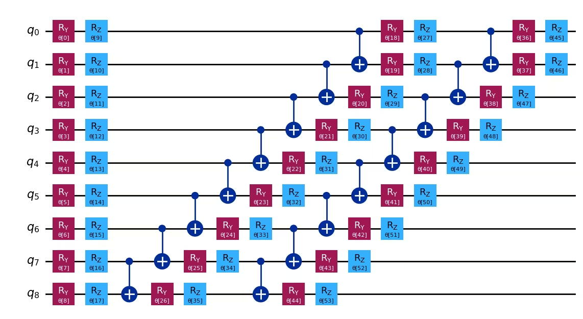
Here, the state $|\psi \rangle$ is parameterized with $\mathbf{\theta}$ , and we optimize these parameters $\mathbf{\theta}$ using a variational approach. This tutorial employs the efficient_su2 ansatz for our variational algorithm due to its expressive capabilities and ease of implementation. We also use the relaxed loss function, which will be introduced later in this tutorial. As a result, we can address large-scale problems with fewer qubits and shallower circuit depths.

# Build the quantum circuit
qc = efficient_su2(num_qubits, su2_gates=["ry", "rz"], reps=2)
qc.draw("mpl")

Output of the previous code cell

# Optimize the circuit

pm = generate_preset_pass_manager(optimization_level=3, backend=backend)
qc = pm.run(qc)

Loss function

For the loss function $\mathcal{L}$ , we use a relaxation of the max-cut objective function as described in [1], which is defined as $\mathcal{V}(\mathbf{x}) \coloneqq \sum_{(i, j) \in E} W_{i, j}(1-x_i x_j)$ . Here, $W_{i, j}$ denotes the weight of the edge $(i, j)$ , and $x_i$ represents the partition of node $i$ . The loss function $\mathcal{L}$ is given by:

$\mathcal{L}\coloneqq \sum_{(i, j) \in E} W_{i, j} \text{tanh} (\alpha \langle\prod_i \rangle) \text{tanh} (\alpha \langle\prod_j \rangle) + \mathcal{L}^{(\text{reg})},$

where the max-cut objective function is replaced by the smooth hyperbolic tangents of the expectation values of the Pauli strings encoding the nodes. The regularization term $\mathcal{L}^{(\text{reg})}$ and the rescaling factor $\alpha$ , proportional to the number of qubits, are introduced to improve the solver's performance.

The regularization term is defined as:

$\mathcal{L}^{(\text{reg})}$ is defined as $\mathcal{L}^{(\text{reg})} \coloneqq \beta \nu \lbrack \frac{1}{m} \sum_{i \in V} \text{tanh} (\alpha \langle\prod_i \rangle)^2 \rbrack ^2$

where $\beta=1/2$ , $\nu = |E|/2 + (m -1) /4$ , $|E|$ is the number of edges, and $m$ is the number of nodes in the graph.

def loss_func_estimator(x, ansatz, hamiltonian, estimator, graph):
    """
    Calculates the specified loss function for the given ansatz, Hamiltonian, and graph.

    The expectation values of each Pauli string in the Hamiltonian are first obtained
    by running the ansatz on the quantum backend. These expectation values are then
    passed through the nonlinear function tanh(alpha * prod_i). The loss function is
    subsequently computed from these transformed values.
    """
    job = estimator.run(
        [
            (ansatz, hamiltonian[0], x),
            (ansatz, hamiltonian[1], x),
            (ansatz, hamiltonian[2], x),
        ]
    )
    result = job.result()

    # calculate the loss function
    node_exp_map = {}
    idx = 0
    for r in result:
        for ev in r.data.evs:
            node_exp_map[idx] = ev
            idx += 1

    loss = 0
    alpha = num_qubits
    for edge0, edge1 in graph.edge_list():
        loss += np.tanh(alpha * node_exp_map[edge0]) * np.tanh(
            alpha * node_exp_map[edge1]
        )

    regulation_term = 0
    for i in range(len(graph.nodes())):
        regulation_term += np.tanh(alpha * node_exp_map[i]) ** 2
    regulation_term = regulation_term / len(graph.nodes())
    regulation_term = regulation_term**2
    beta = 1 / 2
    v = len(graph.edges()) / 2 + (len(graph.nodes()) - 1) / 4
    regulation_term = beta * v * regulation_term

    loss = loss + regulation_term

    global experiment_result
    print(f"Iter {len(experiment_result)}: {loss}")
    experiment_result.append({"loss": loss, "exp_map": node_exp_map})
    return loss

Step 3: Execute using Qiskit primitives

In this tutorial, we set max_iter=50 in the optimization loop for demonstration purposes. If we increase the number of iterations, we can expect better results.

pce = []
pce.append(
    [op.apply_layout(qc.layout) for op in pauli_correlation_encoding_x]
)
pce.append(
    [op.apply_layout(qc.layout) for op in pauli_correlation_encoding_y]
)
pce.append(
    [op.apply_layout(qc.layout) for op in pauli_correlation_encoding_z]
)

max_iter = 50
counter = {"i": 0}
last_x = {"value": None}
last_fun = {"value": None}

with Session(backend=backend) as session:
    estimator = Estimator(mode=session)

    experiment_result = []

    def loss_func(x):
        last_x["value"] = x.copy()
        if counter["i"] + 1 > max_iter:
            return last_fun["value"]
        counter["i"] += 1
        val = loss_func_estimator(
            x, qc, [pce[0], pce[1], pce[2]], estimator, graph
        )
        last_fun["value"] = val
        return val

    np.random.seed(seed)
    initial_params = np.random.rand(qc.num_parameters)

    result = minimize(
        loss_func, initial_params, method="COBYLA", options={"rhobeg": 1.0}
    )

    if counter["i"] >= max_iter:
        result = OptimizeResult(
            message=f"Return from COBYLA because the objective function has been evaluated {max_iter} times.",
            success=False,
            status=3,
            fun=last_fun["value"],
            x=last_x["value"],
            nfev=counter["i"],
        )

print(result)

Iter 0: 159.88755362682548
Iter 1: 113.46202580636677
Iter 2: 56.76494226400048
Iter 3: 32.63357946896002
Iter 4: 21.517837239610117
Iter 5: 30.96034960483569
Iter 6: 20.780475923938027
Iter 7: 24.54251816279811
Iter 8: 27.834486461763042
Iter 9: 16.705460776812693
Iter 10: 18.020587887236864
Iter 11: 12.252379762741352
Iter 12: 5.253885750886939
Iter 13: 6.985984759592262
Iter 14: 6.908717244584757
Iter 15: 12.915466016863858
Iter 16: 4.105776920457279
Iter 17: 11.707504530740305
Iter 18: 7.154360511076546
Iter 19: 10.3890865704735
Iter 20: 10.376147647857252
Iter 21: 2.533430195296697
Iter 22: 3.8612421907795462
Iter 23: 6.103735057461906
Iter 24: -1.1190368234312347
Iter 25: 6.125915279494738
Iter 26: 11.086280445482455
Iter 27: 10.102569882302827
Iter 28: -0.02664415648133822
Iter 29: 7.621887727398785
Iter 30: 5.967346615554497
Iter 31: 3.85345716014828
Iter 32: 4.5494846149011
Iter 33: 10.006668112637232
Iter 34: -3.1927138938527877
Iter 35: 2.8829882366285116
Iter 36: 3.3130087521654144
Iter 37: -4.907566569808272
Iter 38: -4.980134722109894
Iter 39: -2.990457463896541
Iter 40: -5.938401817344579
Iter 41: -2.1807712386469724
Iter 42: -1.0945774380342126
Iter 43: -4.7548102593556685
Iter 44: -3.8762362299208144
Iter 45: -4.9348321021624
Iter 46: -6.487722842864011
Iter 47: 0.7064210113389331
Iter 48: -2.3428323031772216
Iter 49: -2.626032270380895
 message: Return from COBYLA because the objective function has been evaluated 50 times.
 success: False
  status: 3
     fun: -2.626032270380895
       x: [ 1.375e+00  1.951e+00 ...  9.395e-01  8.948e-01]
    nfev: 50

Step 4: Post-process and return result in desired classical format

The partitions of the nodes are determined by evaluating the sign of the expectation values of the Pauli strings that encode the nodes.

# Calculate the partitions based on the final expectation values
# If the expectation value is positive, the node belongs to partition 0 (par0)
# Otherwise, the node belongs to partition 1 (par1)
def get_partitions(experiment_result):
    par0, par1 = set(), set()
    best_index = min(
        range(len(experiment_result)),
        key=lambda i: experiment_result[i]["loss"],
    )
    for i in experiment_result[best_index]["exp_map"]:
        if experiment_result[best_index]["exp_map"][i] >= 0:
            par0.add(i)
        else:
            par1.add(i)
    return par0, par1, best_index

par0, par1, best_index = get_partitions(experiment_result)
print(par0, par1)

{0, 2, 3, 8, 9, 11, 12, 13, 17, 18, 20, 22, 23, 24, 25, 26, 27, 30, 35, 37, 38, 40, 43, 46, 48, 49, 50, 51, 53, 57, 61, 62, 63, 66, 67, 68, 70, 71, 74, 77, 81, 82, 83, 84, 87, 88, 94, 96, 99} {1, 4, 5, 6, 7, 10, 14, 15, 16, 19, 21, 28, 29, 31, 32, 33, 34, 36, 39, 41, 42, 44, 45, 47, 52, 54, 55, 56, 58, 59, 60, 64, 65, 69, 72, 73, 75, 76, 78, 79, 80, 85, 86, 89, 90, 91, 92, 93, 95, 97, 98}

We can calculate the cut size of the max-cut problem using the partitions of the node.

cut_size = calc_cut_size(graph, par0, par1)
print(f"Cut size: {cut_size}")

Cut size: 268

Once the training is complete, we perform one round of single-bit swap search to improve the solution as a classical post-processing step. In this process, we swap the partitions of two nodes and evaluate the cut size. If the cut size is improved, we keep the swap. We repeat this process for all possible pairs of nodes connected by an edge.

cur_bits = []

for i in experiment_result[best_index]["exp_map"]:
    if experiment_result[best_index]["exp_map"][i] >= 0:
        cur_bits.append(1)
    else:
        cur_bits.append(0)
print(cur_bits)

[1, 0, 1, 1, 0, 0, 0, 0, 1, 1, 0, 1, 1, 1, 0, 0, 0, 1, 1, 0, 1, 0, 1, 1, 1, 1, 1, 1, 0, 0, 1, 0, 0, 0, 0, 1, 0, 1, 1, 0, 1, 0, 0, 1, 0, 0, 1, 0, 1, 1, 1, 1, 0, 1, 0, 0, 0, 1, 0, 0, 0, 1, 1, 1, 0, 0, 1, 1, 1, 0, 1, 1, 0, 0, 1, 0, 0, 1, 0, 0, 0, 1, 1, 1, 1, 0, 0, 1, 1, 0, 0, 0, 0, 0, 1, 0, 1, 0, 0, 1]

# Swap the partitions and calculate the cut size

def swap_partitions(graph, cur_bits):
    best_cut = 0
    best_bits = []
    for edge0, edge1 in graph.edge_list():
        swapped_bits = cur_bits.copy()
        swapped_bits[edge0], swapped_bits[edge1] = (
            swapped_bits[edge1],
            swapped_bits[edge0],
        )

        cur_partition = [set(), set()]
        for i, bit in enumerate(swapped_bits):
            if bit > 0:
                cur_partition[0].add(i)
            else:
                cur_partition[1].add(i)
        cut_size = calc_cut_size(graph, cur_partition[0], cur_partition[1])
        if best_cut < cut_size:
            best_cut = cut_size
            best_bits = swapped_bits
    return best_cut, best_bits

best_cut, best_bits = swap_partitions(graph, cur_bits)
print(best_cut, best_bits)

279 [1, 0, 1, 1, 0, 0, 0, 0, 1, 0, 0, 1, 1, 1, 0, 0, 0, 1, 1, 0, 1, 0, 1, 1, 1, 1, 1, 1, 0, 0, 1, 0, 0, 0, 0, 1, 0, 1, 1, 0, 1, 0, 0, 1, 0, 0, 1, 0, 1, 1, 1, 1, 1, 1, 0, 0, 0, 1, 0, 0, 0, 1, 1, 1, 0, 0, 1, 1, 1, 0, 1, 1, 0, 0, 1, 0, 0, 1, 0, 0, 0, 1, 1, 1, 1, 0, 0, 1, 1, 0, 0, 0, 0, 0, 1, 0, 1, 0, 0, 1]

Large-scale hardware example

# -------------------------Step 1-------------------------

num_nodes = 1500  # Number of nodes in graph
graph = rx.undirected_gnp_random_graph(num_nodes, 0.1, seed=seed)
nx_graph = nx.Graph()
nx_graph.add_nodes_from(range(num_nodes))
for edge in graph.edge_list():
    nx_graph.add_edge(edge[0], edge[1])

num_qubits = int(np.ceil((1 + np.sqrt(1 + (8 / 3) * num_nodes)) / 2))

list_size = num_nodes // 3
node_x = [i for i in range(list_size)]
node_y = [i for i in range(list_size, 2 * list_size)]
node_z = [i for i in range(2 * list_size, num_nodes)]

pauli_correlation_encoding_x = build_pauli_correlation_encoding(
    "X", node_x, num_qubits
)
pauli_correlation_encoding_y = build_pauli_correlation_encoding(
    "Y", node_y, num_qubits
)
pauli_correlation_encoding_z = build_pauli_correlation_encoding(
    "Z", node_z, num_qubits
)
print(f"We are using {num_qubits} qubits")

# -------------------------Step 2-------------------------
backend = real_backend
print(f"We are using the {backend.name}")
qc = efficient_su2(num_qubits, ["ry", "rz"], reps=2)
pm = generate_preset_pass_manager(optimization_level=3, backend=backend)
qc = pm.run(qc)
# -------------------------Step 3-------------------------
pce = []
pce.append(
    [op.apply_layout(qc.layout) for op in pauli_correlation_encoding_x]
)
pce.append(
    [op.apply_layout(qc.layout) for op in pauli_correlation_encoding_y]
)
pce.append(
    [op.apply_layout(qc.layout) for op in pauli_correlation_encoding_z]
)

# Run the optimization using a session.
max_iter = 50
counter = {"i": 0}
with Session(backend=backend) as session:
    estimator = Estimator(mode=session)
    estimator.options.environment.job_tags = ["TUT_PCEFQ"]
    experiment_result = []

    def loss_func(x):
        last_x["value"] = x.copy()
        if counter["i"] + 1 > max_iter:
            return last_fun["value"]
        counter["i"] += 1
        val = loss_func_estimator(
            x, qc, [pce[0], pce[1], pce[2]], estimator, graph
        )
        last_fun["value"] = val
        return val

    np.random.seed(seed)
    initial_params = np.random.rand(qc.num_parameters)
    result = minimize(
        loss_func, initial_params, method="COBYLA", options={"rhobeg": 1.0}
    )
    if counter["i"] >= max_iter:
        result = OptimizeResult(
            message=f"Return from COBYLA because the objective function has been evaluated {max_iter} times.",
            success=False,
            status=3,
            fun=last_fun["value"],
            x=last_x["value"],
            nfev=counter["i"],
        )
print(result)

# -------------------------Step 4-------------------------

par0, par1, best_index = get_partitions(experiment_result)
cut_size = calc_cut_size(graph, par0, par1)
print(f"Cut size: {cut_size}")

best_bits = []
cur_bits = []
for i in experiment_result[best_index]["exp_map"]:
    if experiment_result[best_index]["exp_map"][i] >= 0:
        cur_bits.append(1)
    else:
        cur_bits.append(0)
best_cut, best_bits = swap_partitions(graph, cur_bits)
# Print final solution

print(
    f"The best max-cut value achieved for a graph with {num_nodes} nodes on {num_qubits} qubits is {best_cut}"
)
print(f"and the specific partition we obtained is {best_bits}")

We are using 33 qubits
We are using the ibm_pittsburgh
Iter 0: 57399.57543902076
Iter 1: 56458.787143794
Iter 2: 40778.45608998947
Iter 3: 35571.58511146131
Iter 4: 33861.6835761173
Iter 5: 39697.22637736274
Iter 6: 34984.77893767163
Iter 7: 32051.882157096858
Iter 8: 26134.153216063707
Iter 9: 24914.322627065787
Iter 10: 24030.21227315425
Iter 11: 23047.463945514
Iter 12: 22629.42866110748
Iter 13: 17374.859132614685
Iter 14: 18020.11637762458
Iter 15: 17924.7066364044
Iter 16: 15825.1992250984
Iter 17: 16553.346711978447
Iter 18: 12393.565736512377
Iter 19: 11994.021456089155
Iter 20: 11199.994322735669
Iter 21: 9624.895532927634
Iter 22: 9073.811130188606
Iter 23: 9836.721241931278
Iter 24: 10555.925186133794
Iter 25: 9179.1179493286
Iter 26: 8495.394826965305
Iter 27: 8913.688189840399
Iter 28: 7830.448471810181
Iter 29: 7757.430542422075
Iter 30: 6796.187594518731
Iter 31: 7307.985913766867
Iter 32: 7340.225833330675
Iter 33: 7064.731899380469
Iter 34: 7632.270657372515
Iter 35: 7049.154710767935
Iter 36: 7486.118442084411
Iter 37: 6302.12602219333
Iter 38: 6244.934230209166
Iter 39: 7154.9748739261395
Iter 40: 6482.109600054041
Iter 41: 5718.475169152395
Iter 42: 5693.008457857462
Iter 43: 4869.782667921923
Iter 44: 4957.625304450959
Iter 45: 5582.240637063214
Iter 46: 4983.90082772116
Iter 47: 5416.268575648202
Iter 48: 4809.98398457807
Iter 49: 5092.527306646118
 message: Return from COBYLA because the objective function has been evaluated 50 times.
 success: False
  status: 3
     fun: 5092.527306646118
       x: [ 1.375e+00  1.951e+00 ...  7.259e-01  8.971e-01]
    nfev: 50
Cut size: 56152
The best max-cut value achieved for a graph with 1500 nodes on 33 qubits is 56219
and the specific partition we obtained is [1, 0, 0, 0, 1, 1, 0, 1, 1, 0, 0, 0, 0, 0, 1, 1, 0, 1, 0, 0, 1, 0, 0, 1, 1, 1, 0, 1, 1, 0, 1, 0, 1, 1, 0, 0, 0, 0, 0, 1, 0, 1, 0, 0, 1, 0, 0, 0, 1, 0, 1, 1, 1, 1, 0, 1, 0, 0, 1, 0, 0, 0, 0, 1, 1, 0, 0, 0, 0, 1, 1, 1, 1, 1, 0, 0, 0, 1, 0, 0, 1, 1, 0, 0, 1, 1, 1, 1, 1, 1, 0, 0, 0, 1, 0, 0, 0, 0, 1, 0, 1, 1, 1, 1, 1, 0, 1, 0, 0, 1, 0, 0, 0, 0, 0, 0, 1, 0, 0, 0, 1, 0, 1, 1, 1, 1, 0, 1, 1, 1, 1, 0, 0, 0, 1, 0, 0, 0, 1, 1, 0, 1, 1, 0, 1, 0, 0, 1, 1, 1, 1, 1, 1, 0, 1, 0, 1, 0, 0, 0, 0, 0, 0, 1, 0, 1, 0, 0, 1, 1, 1, 0, 1, 0, 1, 0, 0, 1, 1, 0, 1, 0, 1, 0, 0, 0, 1, 0, 1, 0, 1, 1, 1, 1, 1, 0, 1, 0, 1, 1, 1, 1, 1, 1, 0, 0, 0, 0, 0, 1, 0, 1, 0, 0, 1, 1, 0, 0, 1, 0, 1, 0, 1, 0, 0, 0, 0, 0, 1, 1, 0, 0, 0, 0, 0, 1, 1, 0, 0, 1, 1, 1, 1, 1, 1, 1, 0, 1, 1, 1, 1, 0, 1, 1, 0, 1, 0, 0, 1, 1, 1, 0, 1, 0, 1, 1, 1, 0, 1, 0, 0, 0, 1, 1, 1, 1, 1, 1, 0, 1, 0, 0, 0, 0, 1, 1, 1, 1, 1, 1, 1, 0, 0, 1, 1, 1, 1, 0, 1, 0, 0, 1, 1, 1, 0, 1, 0, 1, 1, 1, 1, 0, 1, 1, 0, 1, 0, 0, 0, 0, 0, 0, 0, 0, 0, 0, 1, 0, 0, 0, 0, 0, 0, 1, 1, 1, 0, 0, 1, 1, 1, 0, 1, 0, 1, 0, 1, 0, 1, 1, 1, 0, 0, 1, 1, 1, 0, 1, 0, 0, 0, 1, 1, 1, 0, 0, 0, 1, 0, 1, 0, 0, 0, 0, 1, 1, 0, 0, 1, 1, 1, 1, 0, 1, 0, 1, 0, 0, 1, 1, 0, 0, 1, 1, 0, 0, 0, 1, 1, 1, 0, 1, 1, 0, 0, 0, 1, 1, 1, 0, 0, 1, 1, 1, 1, 1, 0, 0, 1, 1, 0, 0, 0, 0, 0, 0, 1, 1, 1, 1, 1, 1, 1, 0, 0, 0, 1, 1, 0, 0, 0, 1, 0, 0, 1, 0, 0, 1, 0, 1, 1, 0, 0, 0, 0, 0, 0, 0, 1, 1, 1, 1, 1, 0, 0, 0, 1, 0, 0, 1, 1, 1, 1, 1, 1, 1, 1, 1, 1, 1, 0, 1, 0, 1, 1, 1, 1, 1, 0, 0, 0, 1, 1, 1, 0, 1, 1, 1, 1, 0, 0, 1, 0, 1, 0, 1, 1, 0, 0, 0, 1, 0, 1, 0, 1, 1, 1, 0, 1, 0, 1, 1, 0, 1, 1, 0, 1, 1, 1, 0, 0, 1, 1, 1, 0, 1, 0, 1, 0, 1, 0, 0, 0, 1, 1, 0, 1, 0, 0, 1, 0, 0, 1, 0, 0, 0, 0, 0, 1, 0, 0, 0, 0, 0, 1, 0, 0, 0, 0, 0, 0, 0, 0, 1, 0, 1, 0, 0, 1, 0, 1, 0, 0, 0, 0, 1, 0, 0, 0, 1, 1, 1, 1, 1, 0, 0, 1, 0, 1, 1, 1, 1, 0, 1, 1, 0, 1, 0, 0, 0, 0, 1, 0, 0, 1, 1, 0, 1, 0, 1, 0, 1, 0, 0, 1, 0, 0, 0, 1, 1, 1, 0, 0, 1, 0, 0, 1, 0, 1, 0, 1, 1, 1, 1, 0, 1, 1, 1, 0, 1, 1, 1, 1, 1, 1, 1, 1, 0, 1, 0, 1, 1, 1, 0, 0, 0, 1, 0, 0, 0, 0, 0, 1, 0, 0, 1, 0, 1, 1, 1, 0, 0, 0, 0, 0, 0, 1, 0, 1, 1, 0, 1, 1, 1, 1, 0, 0, 1, 1, 0, 1, 1, 1, 0, 1, 0, 1, 0, 1, 0, 0, 0, 0, 0, 0, 0, 0, 1, 0, 0, 1, 1, 1, 0, 1, 1, 0, 0, 0, 1, 0, 1, 0, 1, 1, 1, 0, 1, 1, 1, 0, 1, 1, 1, 1, 0, 0, 1, 1, 0, 1, 1, 1, 0, 0, 0, 0, 0, 0, 0, 1, 1, 1, 1, 1, 0, 1, 0, 1, 0, 1, 0, 0, 0, 1, 0, 1, 0, 1, 0, 1, 0, 1, 0, 1, 1, 1, 1, 1, 0, 0, 1, 0, 1, 0, 1, 0, 1, 1, 0, 1, 0, 1, 0, 0, 0, 1, 0, 0, 0, 1, 1, 1, 0, 1, 0, 0, 1, 0, 1, 0, 1, 0, 1, 0, 0, 1, 0, 1, 0, 0, 0, 1, 1, 1, 0, 1, 0, 0, 0, 0, 1, 0, 0, 0, 0, 1, 0, 0, 1, 1, 1, 0, 1, 1, 0, 1, 1, 1, 0, 0, 0, 0, 1, 0, 1, 0, 0, 0, 1, 0, 1, 0, 1, 0, 0, 1, 0, 1, 0, 1, 0, 1, 1, 0, 0, 1, 1, 0, 1, 1, 0, 0, 1, 0, 1, 1, 1, 0, 1, 1, 0, 1, 1, 1, 0, 1, 1, 0, 1, 0, 1, 0, 1, 1, 0, 1, 1, 0, 1, 1, 0, 0, 0, 1, 0, 1, 0, 0, 0, 0, 0, 1, 0, 0, 1, 1, 0, 1, 0, 1, 1, 0, 1, 1, 0, 1, 1, 1, 1, 0, 1, 0, 1, 1, 0, 0, 1, 0, 0, 1, 1, 0, 1, 1, 1, 0, 1, 1, 0, 1, 1, 1, 0, 1, 0, 0, 0, 1, 0, 0, 1, 1, 1, 0, 0, 1, 0, 1, 1, 1, 0, 1, 0, 1, 1, 1, 1, 1, 1, 0, 1, 0, 0, 0, 1, 0, 1, 0, 1, 1, 0, 0, 0, 1, 1, 0, 1, 1, 1, 1, 1, 1, 1, 1, 1, 1, 1, 1, 0, 1, 1, 1, 0, 0, 0, 0, 1, 0, 0, 0, 0, 1, 1, 1, 0, 0, 1, 0, 0, 0, 0, 0, 0, 0, 1, 0, 0, 0, 0, 0, 0, 0, 1, 1, 0, 0, 1, 0, 0, 1, 1, 0, 1, 0, 1, 0, 1, 0, 0, 1, 1, 0, 1, 1, 1, 0, 0, 1, 1, 1, 1, 1, 0, 0, 1, 0, 1, 1, 1, 1, 0, 1, 0, 1, 1, 0, 0, 1, 0, 1, 0, 0, 1, 0, 1, 1, 1, 1, 1, 1, 1, 0, 1, 0, 1, 1, 0, 0, 0, 0, 0, 1, 1, 0, 0, 1, 1, 1, 1, 1, 1, 1, 1, 1, 1, 0, 1, 1, 1, 1, 0, 1, 0, 0, 0, 1, 1, 1, 1, 0, 0, 0, 1, 1, 0, 0, 0, 0, 0, 1, 0, 0, 0, 1, 0, 0, 0, 1, 1, 1, 1, 0, 0, 0, 1, 1, 1, 1, 1, 1, 1, 1, 1, 1, 0, 1, 1, 1, 1, 1, 1, 1, 0, 0, 0, 0, 0, 1, 1, 0, 0, 0, 1, 1, 0, 0, 0, 0, 0, 1, 0, 0, 0, 0, 0, 0, 0, 0, 1, 0, 1, 0, 1, 1, 1, 0, 1, 0, 1, 1, 1, 1, 1, 0, 1, 1, 1, 1, 0, 1, 1, 1, 1, 1, 1, 0, 0, 1, 1, 0, 0, 1, 1, 1, 1, 1, 0, 1, 0, 1, 1, 1, 1, 1, 0, 1, 0, 0, 1, 1, 0, 0, 0, 0, 1, 1, 1, 1, 0, 1, 1, 1, 1, 1, 1, 1, 1, 0, 0, 0, 1, 0, 1, 1, 0, 1, 0, 1, 1, 1, 1, 0, 1, 1, 1, 1, 1, 1, 1, 1, 0, 1, 1, 0, 0, 0, 0, 0, 0, 1, 1, 0, 0, 0, 0, 0, 0, 1, 0, 0, 0, 0, 0, 0, 0, 0, 0, 0, 1, 0, 0, 0, 0, 0, 0, 0, 1, 0, 0, 1, 0, 0, 0, 0, 0, 0, 0, 0, 0, 0, 0, 0, 0, 0, 1, 1, 1, 0, 1, 1, 1, 1, 1, 0, 1, 0, 1, 1, 0, 1, 1, 1, 1, 1, 1, 1, 1, 1, 1, 0, 1, 1, 1, 1, 1, 1, 1, 0, 1, 0, 1, 0, 1, 1, 1, 1, 1, 1, 1, 1, 1, 1, 0, 0, 1, 1, 1, 1, 0, 1, 0, 1, 1, 1, 1, 1, 1, 1, 0, 0, 1, 1, 1, 0, 0, 1, 0, 1, 1, 1, 1, 0, 1, 1, 1, 1, 1, 1, 0, 1, 1, 0, 1, 1, 0, 1, 1, 1, 1, 1, 1, 1, 1, 1, 0, 1, 1, 1, 1, 0, 1, 1, 1, 1, 1, 1, 1, 1, 1, 1, 1, 1, 1, 1, 1, 1, 1, 1, 1]

Next steps

Recommendations

If you found this work interesting, you might be interested in the following material:

References

[1] Sciorilli, M., Borges, L., Patti, T. L., García-Martín, D., Camilo, G., Anandkumar, A., & Aolita, L. (2024). Towards large-scale quantum optimization solvers with few qubits. arXiv preprint arXiv:2401.09421.

Tutorial survey

Please take this short survey to provide feedback on this tutorial. Your insights will help us improve our content offerings and user experience.

Note: This survey is by IBM Quantum and covers the tutorial content (written by IBM). doQumentation provides the website, translations, and code execution — for feedback on those, please open a GitHub issue.

Learning outcomes​

Prerequisites​

Background​

Overview​

Requirements​

Setup​

Small-scale simulator example​

Step 1: Map classical inputs to a quantum problem​

The max-cut problem​

Graph -> Hamiltonian​

Step 2: Optimize problem for quantum hardware execution​

Quantum circuit​

Loss function​

Step 3: Execute using Qiskit primitives​

Step 4: Post-process and return result in desired classical format​