Krylov quantum diagonalization of lattice Hamiltonians

Usage estimate: 70 minutes on a Heron or Nighthawk processor (NOTE: This is an estimate only. Your runtime might vary.)

Learning outcomes

After completing this tutorial, you can expect to understand the following information:

How to interpret Krylov quantum diagonalization (KQD) as learning a finite Hamiltonian function that acts as a spectral filter.
How to build the projected Hamiltonian and overlap matrices with extended swap-test measurements.
How to solve the resulting generalized eigenvalue problem (GEVP) and recover a ground-state energy estimate for a lattice Hamiltonian.

Prerequisites

It is recommended that you familiarize yourself with these topics:

Background

This tutorial demonstrates how to implement the Krylov quantum diagonalization (KQD) algorithm within the context of Qiskit patterns. You will first learn the theory behind the algorithm and then see a demonstration of its execution on a QPU.

Estimating the low-energy properties of many-body Hamiltonians is a central task in quantum simulation. For example, ground-state energies and low-lying excitations are directly related to chemical stability, magnetic ordering, quantum phase transitions, and material response. On a classical computer, the Hilbert-space dimension grows exponentially with the number of orbitals or spins, so direct diagonalization quickly becomes impractical.

There are several quantum-computing approaches to this problem. Near-term variational methods, such as the variational quantum eigensolver (VQE), use relatively shallow parameterized circuits, but they require a nonlinear classical optimization loop with many quantum-circuit evaluations. At the other end, quantum phase estimation (QPE) provides a more direct route to eigenvalue estimation with rigorous guarantees, but standard QPE requires long coherent circuits and is mainly suited to fault-tolerant quantum computers. KQD sits between these two approaches: it uses real-time Hamiltonian evolution, as in phase-estimation-based algorithms, but replaces full phase estimation with a compact projected eigenvalue problem that can be solved classically.

Consider an $n$ -qubit Hamiltonian $H$ and a reference state $\lvert \psi_{0}\rangle$ . The KQD method builds a Krylov subspace from real-time evolved states,

\begin{equation*} \lvert \psi_\ell\rangle = e^{-i\ell\Delta t H}\lvert \psi_{0}\rangle, \qquad \ell = 0,1,\ldots,r-1, \end{equation*}

where $r$ is the Krylov dimension and $\Delta t$ is the time step. Any state in the Krylov subspace is then represented as a linear combination of these basis states,

\begin{equation*} \lvert \psi(\mathbf{c})\rangle = \frac{\sum_{\ell=0}^{r-1} c_\ell \lvert \psi_\ell\rangle} {\left\|\sum_{\ell=0}^{r-1} c_\ell \lvert \psi_\ell\rangle\right\|}, \end{equation*}

where the denominator normalizes the state.

With simple algebra, we can see that the corresponding energy is written as the Rayleigh quotient,

\begin{equation*} E(\mathbf{c}) =\langle \psi(\mathbf{c})|H|\psi(\mathbf{c}) \rangle= \frac{ \sum_{k,\ell} c_k^* c_\ell \langle \psi_k\vert H\vert\psi_\ell\rangle }{ \sum_{k,\ell} c_k^* c_\ell \langle \psi_k\vert\psi_\ell\rangle } = \frac{ \mathbf{c}^{\dagger}\mathcal{H}\mathbf{c} }{ \mathbf{c}^{\dagger}\mathcal{S}\mathbf{c} }. \end{equation*}

Here, the matrices $\mathcal{S}$ and $\mathcal{H}$ ,

\begin{equation*} \mathcal{S}_{k\ell}=\langle \psi_k\vert\psi_\ell\rangle, \qquad \mathcal{H}_{k\ell}=\langle \psi_k\vert H\vert\psi_\ell\rangle \end{equation*}

define the projected overlap and Hamiltonian matrices. Their entries are estimated using quantum-circuit measurements.

We aim to find the coefficient $\mathbf{c}$ that gives the minimum $E(\mathbf{c})$ :

\begin{equation*} \min_{\mathbf{c}\neq \mathbf{0}} E(\mathbf{c}). \end{equation*}

By the Rayleigh-Ritz theorem, this minimization is equivalent to solving the generalized eigenvalue problem (GEVP),

\begin{equation*} \mathcal{H}\mathbf{c}=E \mathcal{S}\mathbf{c}. \end{equation*}

Note that the dimension $r$ can be small enough for a classical computer to solve the GEVP.

This is the same variational principle used in classical subspace diagonalization, but here the basis states are generated by quantum time evolution. Compared with VQE, KQD usually requires deeper circuits because it relies on real-time evolution. In return, KQD avoids nonlinear parameter optimization and iterative quantum-hardware execution, and it systematically improves as the projected subspace is enlarged. The algorithm has been demonstrated at large scale on existing quantum hardware [2], and its performance can be analyzed with provable guarantees [1].

Requirements

Before starting this tutorial, ensure that you have the following installed:

Qiskit SDK v2.3 or later with visualization support
Qiskit Runtime v0.22 or later (pip install qiskit-ibm-runtime)
SciPy (pip install scipy)
Matplotlib (pip install matplotlib)
Pandas (pip install pandas)

Hardware execution requires qiskit-ibm-runtime and access to an IBM Quantum® account.

Setup

The setup cell imports the required modules and defines helper functions for the workflow:

build the Heisenberg Hamiltonian;
solve the thresholded GEVP;
evaluate the learned Krylov filter;
convert filter values into spectral weights;
plot the reference and filtered energy distributions.

# Added by doQumentation — required packages for this notebook
!pip install -q matplotlib numpy pandas qiskit qiskit-ibm-runtime scipy

from __future__ import annotations

import warnings

import numpy as np
import pandas as pd
import scipy.linalg as la
import matplotlib.pyplot as plt

from qiskit import QuantumCircuit, transpile
from qiskit.circuit import Parameter
from qiskit.circuit.library import PauliEvolutionGate
from qiskit.primitives import StatevectorEstimator
from qiskit.quantum_info import Operator, SparsePauliOp
from qiskit.synthesis import LieTrotter, SuzukiTrotter
from qiskit.transpiler import PassManager, Layout
from qiskit.transpiler.passes import CommutativeOptimization
from qiskit.transpiler.preset_passmanagers import generate_preset_pass_manager
from qiskit_ibm_runtime import QiskitRuntimeService, EstimatorV2, Batch
from qiskit_ibm_runtime.fake_provider import FakeMarrakesh

warnings.filterwarnings("ignore")

def make_heisenberg_hamiltonian(
    num_qubits: int,
    coupling: float = 1.0,
) -> SparsePauliOp:
    """Make a Heisenberg Hamiltonian for a 1D chain of qubits with nearest-neighbor interactions."""
    terms: list[tuple[str, complex]] = []

    def append_term(q0: int, q1: int, pauli: str):
        label = ["I"] * num_qubits
        label[num_qubits - 1 - q0] = pauli[0]
        label[num_qubits - 1 - q1] = pauli[1]
        terms.append(("".join(label), coupling))

    for pauli in ("XX", "YY", "ZZ"):
        for q in range(num_qubits - 1):
            append_term(q, q + 1, pauli)
    return SparsePauliOp.from_list(terms).simplify()

def _basis_state_transition_amplitude_sparse(
    hamiltonian: SparsePauliOp,
    bra_state: int,
    ket_state: int,
) -> complex:
    """Evaluate <bra_state|H|ket_state> for computational-basis states."""
    num_qubits = hamiltonian.num_qubits
    amplitude = 0.0 + 0.0j
    for pauli, coeff in zip(hamiltonian.paulis, hamiltonian.coeffs):
        new_state = ket_state
        phase = 1.0 + 0.0j
        for q in range(num_qubits):
            x = bool(pauli.x[q])
            z = bool(pauli.z[q])
            if not x and not z:
                continue
            bit = (new_state >> q) & 1
            if x and z:
                # Y|0> = i|1>, Y|1> = -i|0>
                phase *= 1j if bit == 0 else -1j
                new_state ^= 1 << q
            elif x:
                new_state ^= 1 << q
            else:
                # Z|0> = |0>, Z|1> = -|1>
                if bit:
                    phase *= -1
        if new_state == bra_state:
            amplitude += coeff * phase
    return amplitude

def basis_state_expectation_sparse(
    hamiltonian: SparsePauliOp,
    bitstring: str,
) -> complex:
    """Evaluate <bitstring|H|bitstring>."""
    state = int(bitstring, 2)
    return _basis_state_transition_amplitude_sparse(
        hamiltonian,
        bra_state=state,
        ket_state=state,
    )

def diagonalize_single_1_subspace(
    hamiltonian: SparsePauliOp,
) -> np.ndarray:
    """Diagonalize the Hamiltonian projected onto the single-excitation subspace."""
    num_qubits = hamiltonian.num_qubits

    # Integer basis states |...010...>, with the excitation at qubit k.
    basis = [1 << k for k in range(num_qubits)]

    h_single = np.empty((num_qubits, num_qubits), dtype=complex)

    for row, bra_state in enumerate(basis):
        for col, ket_state in enumerate(basis):
            h_single[row, col] = _basis_state_transition_amplitude_sparse(
                hamiltonian,
                bra_state=bra_state,
                ket_state=ket_state,
            )
    # Remove floating-point-level asymmetry.
    h_single = 0.5 * (h_single + h_single.conj().T)
    evals, _ = np.linalg.eigh(h_single)
    return np.real(evals)

def simple_transpilation(circuit: QuantumCircuit) -> QuantumCircuit:
    """Transpilation to simplify the circuit"""
    pm = PassManager(
        [
            CommutativeOptimization(),
        ]
    )
    circuit = transpile(circuit, optimization_level=3)
    circuit = pm.run(circuit)
    return circuit

def summarize_circuit(circuit: QuantumCircuit) -> dict[str, int | str]:
    """Summarize the circuit with depth, size, and 2-qubit gate information."""
    two_qubit_total = sum(
        inst.operation.num_qubits == 2 for inst in circuit.data
    )
    two_qubit_depth = circuit.depth(lambda x: x[0].num_qubits == 2)
    return {
        "depth": circuit.depth(),
        "size": circuit.size(),
        "2q gates": two_qubit_total,
        "2q depth": two_qubit_depth,
    }

def solve_thresholded_gevp(
    h_matrix: np.ndarray,
    s_matrix: np.ndarray,
    threshold: float = 1e-10,
) -> tuple[float, np.ndarray, int]:
    """Solve H c = E S c using canonical orthogonalization of S."""
    s_vals, s_vecs = la.eigh(s_matrix)

    valid = s_vals > threshold
    if not np.any(valid):
        raise ValueError(
            "All overlap eigenvalues were removed by thresholding."
        )

    keep = valid

    orthogonalizer = s_vecs[:, keep] @ np.diag(1.0 / np.sqrt(s_vals[keep]))
    h_orth = orthogonalizer.conj().T @ h_matrix @ orthogonalizer
    h_orth = 0.5 * (h_orth + h_orth.conj().T)

    eigvals, eigvecs = la.eigh(h_orth)

    coeffs = orthogonalizer @ eigvecs[:, 0]
    normalization = np.sqrt(np.real(coeffs.conj().T @ s_matrix @ coeffs))
    coeffs /= normalization

    return float(np.real(eigvals[0])), coeffs, int(np.sum(keep))

In the first part of this tutorial, we demonstrate the KQD method by using a local statevector simulator. Later, we use a real quantum backend to address a utility-scale problem.

We also define a fake backend to demonstrate backend-specific transpilation and inspect the resulting circuit.

try:
    service = QiskitRuntimeService()
except Exception:
    QiskitRuntimeService.save_account(
        token="<api_token>", instance="<instance>", overwrite=True
    )
    service = QiskitRuntimeService()

backend = FakeMarrakesh()

Small-scale simulator example

Step 1: Map classical inputs to a quantum problem

Hamiltonian and reference state

This example uses a 12-qubit open-boundary Heisenberg chain ( $n=12$ ),

\begin{equation*} H=\sum_{i=0}^{n-2}\left(X_iX_{i+1}+Y_iY_{i+1}+Z_iZ_{i+1}\right), \end{equation*}

with a single-excitation product state

\begin{equation*} |\psi_{0}\rangle=|000001000000\rangle \end{equation*}

as the reference state. Because the Heisenberg Hamiltonian defined above conserves the total number of excitations, the reference state stays in the single-excitation subspace, whose dimension grows only linearly with the number of qubits. We can therefore compute the exact ground-state energy efficiently, by diagonalizing the Hamiltonian restricted to that subspace, and use it purely as a diagnostic benchmark for the KQD estimate. The KQD workflow itself estimates projected matrix elements by using Qiskit primitives and solves the resulting projected problem classically.

# Problem definition for the simulator example
num_qubits = 12
hamiltonian = make_heisenberg_hamiltonian(num_qubits=num_qubits, coupling=1.0)
ref_bitstring = "000001000000"
ref_energy = basis_state_expectation_sparse(hamiltonian, ref_bitstring)

print("Hamiltonian:")
print(hamiltonian)
print(f"Reference state: |{ref_bitstring}>")
print("Reference energy: ", ref_energy)

Hamiltonian:
SparsePauliOp(['IIIIIIIIIIXX', 'IIIIIIIIIXXI', 'IIIIIIIIXXII', 'IIIIIIIXXIII', 'IIIIIIXXIIII', 'IIIIIXXIIIII', 'IIIIXXIIIIII', 'IIIXXIIIIIII', 'IIXXIIIIIIII', 'IXXIIIIIIIII', 'XXIIIIIIIIII', 'IIIIIIIIIIYY', 'IIIIIIIIIYYI', 'IIIIIIIIYYII', 'IIIIIIIYYIII', 'IIIIIIYYIIII', 'IIIIIYYIIIII', 'IIIIYYIIIIII', 'IIIYYIIIIIII', 'IIYYIIIIIIII', 'IYYIIIIIIIII', 'YYIIIIIIIIII', 'IIIIIIIIIIZZ', 'IIIIIIIIIZZI', 'IIIIIIIIZZII', 'IIIIIIIZZIII', 'IIIIIIZZIIII', 'IIIIIZZIIIII', 'IIIIZZIIIIII', 'IIIZZIIIIIII', 'IIZZIIIIIIII', 'IZZIIIIIIIII', 'ZZIIIIIIIIII'],
              coeffs=[1.+0.j, 1.+0.j, 1.+0.j, 1.+0.j, 1.+0.j, 1.+0.j, 1.+0.j, 1.+0.j, 1.+0.j,
 1.+0.j, 1.+0.j, 1.+0.j, 1.+0.j, 1.+0.j, 1.+0.j, 1.+0.j, 1.+0.j, 1.+0.j,
 1.+0.j, 1.+0.j, 1.+0.j, 1.+0.j, 1.+0.j, 1.+0.j, 1.+0.j, 1.+0.j, 1.+0.j,
 1.+0.j, 1.+0.j, 1.+0.j, 1.+0.j, 1.+0.j, 1.+0.j])
Reference state: |000001000000>
Reference energy:  (7+0j)

Set the parameters for the algorithm

Based on the upper-bounds on the Hamiltonian norm, Ref. [1] heuristically suggests the time step $\Delta t$ as $\pi/\|H\|$ . Because the spectral norm $\|H\|$ is hard to compute, we instead use its upper bound:

\begin{equation*} \|H\| \le \sum_{i=0}^{n-2}\underbrace{\|X_i X_{i+1}+Y_{i} Y_{i+1}+Z_{i} Z_{i+1}\|}_{4 \times 4 \text{ matrix, easy to calculate the norm}} = 3(n-1). \end{equation*}

We set the Krylov dimension to $r=10$ and the number of Trotter steps per time step to $5$ : a large enough Krylov space to resolve the low-lying spectrum while keeping the deepest circuit ( $t_{\max}=(r-1)\Delta t$ ) affordable, and enough Trotter steps to keep the discretization error small at that deepest circuit.

dt = np.pi / (3 * (num_qubits - 1))
print("dt in Krylov basis:  ", dt)

krylov_dim = 10
num_trotter_steps = 5

dt in Krylov basis:   0.09519977738150888

Build circuit

Here, we build the circuits to estimate the matrix elements $\mathcal{H}_{k\ell}$ and $\mathcal{S}_{k\ell}$ . Because all powers of $H$ commute, we have

\begin{equation*} \mathcal{H}_{k\ell} = \langle\psi_{0}|H e^{-i(\ell-k)\Delta tH}|\psi_{0}\rangle=\mathcal{H}_{0,\ell-k}, \qquad \mathcal{S}_{k\ell} = \langle\psi_{0}|e^{-i(\ell-k)\Delta tH}|\psi_{0}\rangle=\mathcal{S}_{0,\ell-k}. \end{equation*}

Such matrices where the elements depend on the index differences in this manner are called Toeplitz and can be reconstructed from first-row elements indexed by $d=\ell-k$ .

Here, we present the circuit, called extended-swap-test, which prepares

\begin{equation*} |\Phi_{0d}\rangle= \frac{|0\rangle|\psi_0\rangle+|1\rangle|\psi_d\rangle}{\sqrt{2}}, \end{equation*}

where $|\psi_d\rangle=e^{-id\Delta tH}|\psi_{0}\rangle$ .

Reference state

We prepare the reference state $|\psi_0\rangle$ .

qc_ref = QuantumCircuit(num_qubits)
for i, b in enumerate(reversed(ref_bitstring)):
    if b == "1":
        qc_ref.x(i)
display(qc_ref.draw("mpl", scale=0.5))

Output of the previous code cell

Time evolution

Realize the time-evolution operator generated by the Hamiltonian, approximated by simple Lie-Trotterization.

t = Parameter("t")

evol_gate = PauliEvolutionGate(
    hamiltonian,
    time=t,
    synthesis=LieTrotter(reps=num_trotter_steps),
    label="U(t)",
)

# Synthesize U(t) first and then control the synthesized circuit.
# This makes the controlled structure visible in the circuit drawer.
evolution_circuit = QuantumCircuit(num_qubits, name="U(t)")
evolution_circuit.append(evol_gate, range(num_qubits))
evolution_circuit = simple_transpilation(evolution_circuit)

# Make a controlled version of the evolution circuit.
controlled_evolution_gate = evolution_circuit.to_gate(label="U(t)").control(
    1, label="C-U(t)"
)
display(
    evolution_circuit.assign_parameters({t: 1.5}).draw(
        "mpl", scale=0.5, fold=-1
    )
)

Output of the previous code cell

Extended swap test circuit [3]

The circuit first prepares the reference state on the system register while the ancilla remains in $|0\rangle$ :

\begin{equation*} |0\rangle |0\rangle^{\otimes n} \longrightarrow |0\rangle |\psi_{0}\rangle . \end{equation*}

Then, applying a Hadamard gate to the ancilla creates a coherent superposition of two branches:

\begin{equation*} |0\rangle |\psi_0\rangle \longrightarrow \frac{|0\rangle + |1\rangle}{\sqrt{2}} |\psi_0\rangle = \frac{|0\rangle|\psi_0\rangle + |1\rangle|\psi_0\rangle}{\sqrt{2}} . \end{equation*}

Finally, the controlled time-evolution gate applies:

\begin{equation*} U(t=d\Delta t) = e^{-id\Delta t H} \end{equation*}

only when the ancilla is in the $|1\rangle$ branch. Therefore,

\begin{equation*} \frac{|0\rangle|\psi_0\rangle + |1\rangle|\psi_0\rangle}{\sqrt{2}} \longrightarrow \frac{|0\rangle|\psi_0\rangle + |1\rangle U(d\Delta t)|\psi_0\rangle}{\sqrt{2}} . \end{equation*}

In the next code block, we implement:

\begin{equation*} |\Psi(t)\rangle = \frac{|0\rangle|\psi_0\rangle + |1\rangle U(t)|\psi_0\rangle}{\sqrt{2}}, \end{equation*}

which will be assigned as $t=d\Delta t$ for $d=1,\cdots r-1$ in the execution step.

ancilla = 0
system_qubits = list(range(1, num_qubits + 1))

extended_swap_test = QuantumCircuit(num_qubits + 1)

# Append state preparation part
extended_swap_test = extended_swap_test.compose(qc_ref, system_qubits)

# Prepare the coherent branch label, (|0> + |1>) / sqrt(2).
extended_swap_test.h(ancilla)

# Apply U(t) only to the |1> branch of the ancilla.
extended_swap_test.append(
    controlled_evolution_gate, [ancilla] + system_qubits
)

# Decompose once more for visualization so that control bullets are visible.
display(extended_swap_test.draw("mpl", fold=-1))

Output of the previous code cell

Observables

For any Hermitian system observable $O$ , here we set the observables to calculate:

\begin{equation*} z=\langle \psi_0|O|\psi_d\rangle . \end{equation*}

This is because $O=I$ gives the overlap element $\mathcal{S}_{0d}=\langle\psi_0|\psi_d\rangle$ , while $O=H$ gives the Hamiltonian element $\mathcal{H}_{0d}=\langle\psi_0|H|\psi_d\rangle$ .

Using $X=|0\rangle\langle 1|+|1\rangle\langle 0|$ , we have

\begin{align*} \langle \Psi_{0d}|X\otimes O| \Psi_{0d} \rangle &= \left(\frac{\langle0|\langle\psi_0| + \langle1| \langle\psi_d|}{\sqrt{2}}\right)(X\otimes O)\left(\frac{|0\rangle|\psi_0\rangle + |1\rangle |\psi_d\rangle}{\sqrt{2}}\right) \\ &= \frac{1}{2} \left( \langle \psi_0|O|\psi_d\rangle + \langle \psi_d|O|\psi_0\rangle \right) \\ &= \frac{z+z^*}{2} = \operatorname{Re} z. \end{align*}

Similarly, using $Y=-i|0\rangle\langle 1|+i|1\rangle\langle 0|$ ,

\begin{align*} \langle \Psi_{0d}|Y\otimes O| \Psi_{0d} \rangle &= \left(\frac{\langle0|\langle\psi_0| + \langle1| \langle\psi_d|}{\sqrt{2}}\right)(Y\otimes O)\left(\frac{|0\rangle|\psi_0\rangle + |1\rangle |\psi_d\rangle}{\sqrt{2}}\right) \\ &= \frac{1}{2} \left( -i\langle \psi_0|O|\psi_d\rangle + i\langle \psi_d|O|\psi_0\rangle \right) \\ &= \frac{-iz+iz^*}{2} = \operatorname{Im} z. \end{align*}

Therefore, we have

\begin{equation*} \langle \Phi_{0d}|X\otimes O|\Phi_{0d}\rangle = \operatorname{Re}\langle\psi_0|O|\psi_d\rangle , \quad \langle \Phi_{0d}|Y\otimes O|\Phi_{0d}\rangle = \operatorname{Im}\langle\psi_0|O|\psi_d\rangle . \end{equation*}

Finally, for each state $|\Psi_{0d}\rangle$ , we need to measure:

\begin{align*} X \otimes I \text{ for } \operatorname{Re}\mathcal{S}_{0d},\\ Y \otimes I \text{ for } \operatorname{Im}\mathcal{S}_{0d},\\ X \otimes H \text{ for } \operatorname{Re}\mathcal{H}_{0d},\\ Y \otimes H \text{ for } \operatorname{Im}\mathcal{H}_{0d}.\\ \end{align*}

n_qubits = hamiltonian.num_qubits

observable_labels = [
    "Re S_0d",
    "Im S_0d",
    "Re H_0d",
    "Im H_0d",
]

# X ⊗ I and Y ⊗ I.
# Qiskit's Pauli-label convention places qubit 0 on the rightmost character,
# so the ancilla Pauli is appended to the right.
obs_x_identity = SparsePauliOp("I" * n_qubits + "X")
obs_y_identity = SparsePauliOp("I" * n_qubits + "Y")

# X ⊗ H and Y ⊗ H.
obs_x_hamiltonian = SparsePauliOp.from_list(
    [
        (label + "X", coeff)
        for label, coeff in zip(
            hamiltonian.paulis.to_labels(),
            hamiltonian.coeffs,
        )
    ]
)

obs_y_hamiltonian = SparsePauliOp.from_list(
    [
        (label + "Y", coeff)
        for label, coeff in zip(
            hamiltonian.paulis.to_labels(),
            hamiltonian.coeffs,
        )
    ]
)

observables = [
    obs_x_identity,
    obs_y_identity,
    obs_x_hamiltonian,
    obs_y_hamiltonian,
]

for obs, label in zip(observables, observable_labels):
    print(f"Observable: {label}")
    print(obs)
    print()

Observable: Re S_0d
SparsePauliOp(['IIIIIIIIIIIIX'],
              coeffs=[1.+0.j])

Observable: Im S_0d
SparsePauliOp(['IIIIIIIIIIIIY'],
              coeffs=[1.+0.j])

Observable: Re H_0d
SparsePauliOp(['IIIIIIIIIIXXX', 'IIIIIIIIIXXIX', 'IIIIIIIIXXIIX', 'IIIIIIIXXIIIX', 'IIIIIIXXIIIIX', 'IIIIIXXIIIIIX', 'IIIIXXIIIIIIX', 'IIIXXIIIIIIIX', 'IIXXIIIIIIIIX', 'IXXIIIIIIIIIX', 'XXIIIIIIIIIIX', 'IIIIIIIIIIYYX', 'IIIIIIIIIYYIX', 'IIIIIIIIYYIIX', 'IIIIIIIYYIIIX', 'IIIIIIYYIIIIX', 'IIIIIYYIIIIIX', 'IIIIYYIIIIIIX', 'IIIYYIIIIIIIX', 'IIYYIIIIIIIIX', 'IYYIIIIIIIIIX', 'YYIIIIIIIIIIX', 'IIIIIIIIIIZZX', 'IIIIIIIIIZZIX', 'IIIIIIIIZZIIX', 'IIIIIIIZZIIIX', 'IIIIIIZZIIIIX', 'IIIIIZZIIIIIX', 'IIIIZZIIIIIIX', 'IIIZZIIIIIIIX', 'IIZZIIIIIIIIX', 'IZZIIIIIIIIIX', 'ZZIIIIIIIIIIX'],
              coeffs=[1.+0.j, 1.+0.j, 1.+0.j, 1.+0.j, 1.+0.j, 1.+0.j, 1.+0.j, 1.+0.j, 1.+0.j,
 1.+0.j, 1.+0.j, 1.+0.j, 1.+0.j, 1.+0.j, 1.+0.j, 1.+0.j, 1.+0.j, 1.+0.j,
 1.+0.j, 1.+0.j, 1.+0.j, 1.+0.j, 1.+0.j, 1.+0.j, 1.+0.j, 1.+0.j, 1.+0.j,
 1.+0.j, 1.+0.j, 1.+0.j, 1.+0.j, 1.+0.j, 1.+0.j])

Observable: Im H_0d
SparsePauliOp(['IIIIIIIIIIXXY', 'IIIIIIIIIXXIY', 'IIIIIIIIXXIIY', 'IIIIIIIXXIIIY', 'IIIIIIXXIIIIY', 'IIIIIXXIIIIIY', 'IIIIXXIIIIIIY', 'IIIXXIIIIIIIY', 'IIXXIIIIIIIIY', 'IXXIIIIIIIIIY', 'XXIIIIIIIIIIY', 'IIIIIIIIIIYYY', 'IIIIIIIIIYYIY', 'IIIIIIIIYYIIY', 'IIIIIIIYYIIIY', 'IIIIIIYYIIIIY', 'IIIIIYYIIIIIY', 'IIIIYYIIIIIIY', 'IIIYYIIIIIIIY', 'IIYYIIIIIIIIY', 'IYYIIIIIIIIIY', 'YYIIIIIIIIIIY', 'IIIIIIIIIIZZY', 'IIIIIIIIIZZIY', 'IIIIIIIIZZIIY', 'IIIIIIIZZIIIY', 'IIIIIIZZIIIIY', 'IIIIIZZIIIIIY', 'IIIIZZIIIIIIY', 'IIIZZIIIIIIIY', 'IIZZIIIIIIIIY', 'IZZIIIIIIIIIY', 'ZZIIIIIIIIIIY'],
              coeffs=[1.+0.j, 1.+0.j, 1.+0.j, 1.+0.j, 1.+0.j, 1.+0.j, 1.+0.j, 1.+0.j, 1.+0.j,
 1.+0.j, 1.+0.j, 1.+0.j, 1.+0.j, 1.+0.j, 1.+0.j, 1.+0.j, 1.+0.j, 1.+0.j,
 1.+0.j, 1.+0.j, 1.+0.j, 1.+0.j, 1.+0.j, 1.+0.j, 1.+0.j, 1.+0.j, 1.+0.j,
 1.+0.j, 1.+0.j, 1.+0.j, 1.+0.j, 1.+0.j, 1.+0.j])

For the estimation of the $\mathcal{H}$ matrix elements, the number of Pauli terms is much larger than that for the $\mathcal{S}$ matrix elements.

We can now reduce the number of measured Hamiltonian terms by using a shifting technique [4]. We split the Hamiltonian as:

\begin{equation*} H = (H-T) + T, \end{equation*}

where $T$ is chosen such that the reference state is its eigenstate,

\begin{equation*} T|\psi_0\rangle = \tau |\psi_0\rangle . \end{equation*}

Then,

\begin{align*} \mathcal{H}_{0d} &= \langle\psi_0|H|\psi_d\rangle \\ &= \langle\psi_0|(H-T)|\psi_d\rangle + \langle\psi_0|T|\psi_d\rangle \\ &= \langle\psi_0|(H-T)|\psi_d\rangle + \tau \langle\psi_0|\psi_d\rangle \\ &= \widetilde{\mathcal{H}}_{0d} + \tau \mathcal{S}_{0d}. \end{align*}

Here,

\begin{equation*} \widetilde{\mathcal{H}}_{0d} = \langle\psi_0|(H-T)|\psi_d\rangle \end{equation*}

is the shifted Hamiltonian matrix element. Therefore, we only need to measure $X\otimes (H-T)$ and $Y\otimes (H-T)$ . The contribution from $T$ is reconstructed classically using the already measured overlap matrix element $\mathcal{S}_{0d}$ .

In this example, a natural choice is the diagonal part of the Heisenberg Hamiltonian,

\begin{equation*} T = \sum_{i=0}^{n-2} Z_iZ_{i+1}. \end{equation*}

Because the reference state is a computational-basis state, it is an eigenstate of every $Z_iZ_{i+1}$ term.

However, a more advantageous choice is to include not only the diagonal $ZZ$ terms, but also the $XX+YY$ terms that annihilate the reference state.

For each neighboring pair, the operator $XX+YY$ satisfies

\begin{equation*} (XX+YY)|00\rangle = 0, \qquad (XX+YY)|11\rangle = 0, \end{equation*}

and

\begin{equation*} (XX+YY)|01\rangle = 2|10\rangle, \qquad (XX+YY)|10\rangle = 2|01\rangle . \end{equation*}

Therefore, the $XX+YY$ term contributes only when the two neighboring qubits have different occupations in the reference bitstring. If the two qubits are both $0$ or both $1$ , the term annihilates the reference state and can also be shifted out.

Let $|\psi_{\rm ref}\rangle = |z_0\cdots z_{n-1}\rangle$ , where $z_i \in \{0,1\}$ . Thus, we can choose

\begin{equation*} T=\sum_{i=0}^{n-2} Z_iZ_{i+1} + \sum_{z_i={z_{i+1}}} \left( X_iX_{i+1} + Y_iY_{i+1} \right). \end{equation*}

This operator still satisfies

\begin{equation*} T|\psi_0\rangle = \tau |\psi_0\rangle , \end{equation*}

because the $ZZ$ terms act diagonally on $|\psi_0\rangle$ , while the shifted $XX+YY$ terms give zero. The corresponding eigenvalue is therefore determined only by the $ZZ$ terms,

\begin{equation*} \tau = \sum_{i=0}^{n-2} (-1)^{z_i} (-1)^{z_{i+1}} . \end{equation*}

With this choice, the shifted Hamiltonian becomes:

\begin{equation*} H-T = \sum_{z_i\ne z_{i+1}} \left( X_iX_{i+1} + Y_iY_{i+1} \right). \end{equation*}

As a result, only the edges with different occupations in the reference state need to be measured. All $ZZ$ terms and all inactive $XX+YY$ terms are reconstructed through the overlap contribution $\tau \mathcal{S}_{0d}$ , or give zero contribution by construction.

This gives a smaller observable than shifting only the diagonal part. In particular, for a computational-basis reference state with a localized excitation, only the edges adjacent to the excitation remain in $H-T$ . Therefore, the number of Pauli terms in $X\otimes(H-T)$ and $Y\otimes(H-T)$ can be substantially reduced, while the reconstructed matrix element

\begin{equation*} \widetilde{\mathcal{H}}_{0d} + \tau \mathcal{S}_{0d} \end{equation*}

remains exactly the same.

def make_reduced_heisenberg_observables(
    ref_bitstring: str,
    coupling: float = 1.0,
) -> tuple[SparsePauliOp, SparsePauliOp, float]:
    """Build X⊗(H-T), Y⊗(H-T), and tau."""
    n_qubits = len(ref_bitstring)

    shifted_terms: list[tuple[str, complex]] = []
    tau = 0.0

    def bit(q: int) -> str:
        return ref_bitstring[n_qubits - 1 - q]

    def append_term(q0: int, q1: int, pauli: str):
        label = ["I"] * n_qubits
        label[n_qubits - 1 - q0] = pauli[0]
        label[n_qubits - 1 - q1] = pauli[1]
        shifted_terms.append(("".join(label), coupling))

    for q in range(n_qubits - 1):
        same_occupation = bit(q) == bit(q + 1)

        # ZZ contribution to tau
        tau += coupling * (1.0 if same_occupation else -1.0)

        # XX + YY survives only for opposite occupations.
        if not same_occupation:
            append_term(q, q + 1, "XX")
            append_term(q, q + 1, "YY")

    if shifted_terms:
        obs_x_shifted_hamiltonian = SparsePauliOp.from_list(
            [(label + "X", coeff) for label, coeff in shifted_terms]
        )
        obs_y_shifted_hamiltonian = SparsePauliOp.from_list(
            [(label + "Y", coeff) for label, coeff in shifted_terms]
        )
    else:
        obs_x_shifted_hamiltonian = SparsePauliOp(
            "I" * n_qubits + "X", coeffs=[0.0]
        )
        obs_y_shifted_hamiltonian = SparsePauliOp(
            "I" * n_qubits + "Y", coeffs=[0.0]
        )

    return obs_x_shifted_hamiltonian, obs_y_shifted_hamiltonian, tau

obs_x_shifted_hamiltonian, obs_y_shifted_hamiltonian, shift_tau = (
    make_reduced_heisenberg_observables(ref_bitstring)
)

print("Observable: Re shifted H_0d")
print(obs_x_shifted_hamiltonian)
print()

print("Observable: Im shifted H_0d")
print(obs_y_shifted_hamiltonian)
print()

print("tau =", shift_tau)

observables = [
    obs_x_identity,
    obs_y_identity,
    obs_x_shifted_hamiltonian,
    obs_y_shifted_hamiltonian,
]
observable_labels = [
    "Re S_0d",
    "Im S_0d",
    "Re shifted H_0d",
    "Im shifted H_0d",
]

Observable: Re shifted H_0d
SparsePauliOp(['IIIIIXXIIIIIX', 'IIIIIYYIIIIIX', 'IIIIXXIIIIIIX', 'IIIIYYIIIIIIX'],
              coeffs=[1.+0.j, 1.+0.j, 1.+0.j, 1.+0.j])

Observable: Im shifted H_0d
SparsePauliOp(['IIIIIXXIIIIIY', 'IIIIIYYIIIIIY', 'IIIIXXIIIIIIY', 'IIIIYYIIIIIIY'],
              coeffs=[1.+0.j, 1.+0.j, 1.+0.j, 1.+0.j])

tau = 7.0

Step 2: Optimize problem for quantum hardware execution

Now we turn the abstract extended-swap-test circuit into a hardware-oriented template. Before that, we further optimize the circuit in the abstract level first.

Compare Hamiltonian term ordering

First, we compare different orderings of the Pauli terms in the Heisenberg Hamiltonian for the Hamiltonian simulation. The Hamiltonian itself is unchanged, but the ordering affects how the product-formula circuit is generated and how much the structure can be parallelized in the circuit. For example, the naive ordering lists all nearest-neighbor $XX$ terms, then all $YY$ terms, then all $ZZ$ terms. This places adjacent edges such as $(0,1)$ and $(1,2)$ next to each other, so they cannot be executed in parallel. The even-then-odd ordering visits disjoint even edges first, followed by odd edges, which exposes parallel two-qubit layers. The even-odd edge-grouped ordering goes one step further: for each edge, it keeps the local $XX$ , $YY$ , and $ZZ$ terms together, while still visiting even edges before odd edges. We expect the even-then-odd and even-odd edge-grouped orderings to reduce circuit depth by exposing parallel two-qubit layers, and the edge-grouped ordering to additionally reduce the Trotter error because the local two-qubit interaction on the same edge is handled as a compact block.

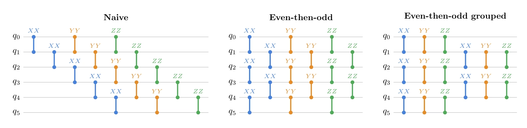
Pauli evolutions with different term ordering

The Hamiltonian ordering also affects the Trotter error. If we place noncommuting terms next to each other, the basis transitions occur more often, which induces more Trotter error. By grouping terms that require the same Pauli-basis transformation, redundant basis-changes can be avoided.

Here, the comparison uses the largest evolution time that appears in the first-row Krylov estimates, $t_{\max} = (r-1)\Delta t,$ using the same transpilation condition.

In order to measure the Trotter error, we use process infidelity between the Trotterized circuit and the exact Hamiltonian evolution,

\begin{equation*} \text{Infidelity}(U,V) = 1-F(U,V) = 1 - \frac{|\operatorname{Tr}(U^\dagger V)|^2}{d^2}, \end{equation*}

where $d=2^n$ is the dimension of the Hilbert space.

This diagnostic uses dense matrices, so it is suitable for this small 12-qubit example but not intended as a scalable subroutine.

# The comparison uses the largest time that appears in the first-row Krylov estimates.
# Circuit depth does not depend on this numeric value, but the Trotter error does.
comparison_time = (krylov_dim - 1) * dt

def make_heisenberg_hamiltonian_ordered(
    num_qubits: int,
    ordering: str,
    coupling: float = 1.0,
) -> SparsePauliOp:
    """Return the same Heisenberg Hamiltonian with a specified term ordering."""
    terms: list[tuple[str, complex]] = []
    even_edges = [(q, q + 1) for q in range(0, num_qubits - 1, 2)]
    odd_edges = [(q, q + 1) for q in range(1, num_qubits - 1, 2)]

    def append_term(q0: int, q1: int, pauli: str):
        label = ["I"] * num_qubits
        label[num_qubits - 1 - q0] = pauli[0]
        label[num_qubits - 1 - q1] = pauli[1]
        terms.append(("".join(label), coupling))

    if ordering == "naive":
        for pauli in ("XX", "YY", "ZZ"):
            for q in range(num_qubits - 1):
                append_term(q, q + 1, pauli)
    elif ordering == "even-then-odd":
        for pauli in ("XX", "YY", "ZZ"):
            for q0, q1 in even_edges + odd_edges:
                append_term(q0, q1, pauli)
    elif ordering == "even-odd edge-grouped":
        for q0, q1 in even_edges + odd_edges:
            for pauli in ("XX", "YY", "ZZ"):
                append_term(q0, q1, pauli)
    else:
        raise ValueError(f"Unknown ordering: {ordering}")

    return SparsePauliOp.from_list(terms).simplify()

def build_numeric_evolution_circuit(
    hamiltonian: SparsePauliOp,
    synthesis,
    time_value: float,
    **synthesis_kwargs,
) -> QuantumCircuit:
    """Build a numeric circuit for exp(-i H t) with a chosen synthesis rule."""
    evolution_gate = PauliEvolutionGate(
        hamiltonian,
        time=time_value,
        synthesis=synthesis(**synthesis_kwargs),
    )
    circuit = QuantumCircuit(hamiltonian.num_qubits)
    circuit.append(evolution_gate, range(hamiltonian.num_qubits))
    return circuit

def process_infidelity(
    circuit: QuantumCircuit,
    exact_matrix: np.ndarray,
) -> float:
    """Return 1 - |Tr(U_circuit† U_exact) / d|²."""
    circuit_matrix = np.asarray(Operator(circuit).data)
    dim = circuit_matrix.shape[0]
    normalized_trace = np.vdot(circuit_matrix, exact_matrix) / dim
    fidelity = np.abs(normalized_trace) ** 2
    return float(np.clip(1.0 - fidelity, 0.0, 1.0))

hamiltonians_by_ordering = {
    ordering: make_heisenberg_hamiltonian_ordered(
        num_qubits, ordering, coupling=1.0
    )
    for ordering in ["naive", "even-then-odd", "even-odd edge-grouped"]
}

print(f"Comparison time: {comparison_time}\n")

for order_name, ham_ordered in hamiltonians_by_ordering.items():
    print(f"{order_name}:")
    print([op for op, _ in ham_ordered.to_list()])
    print()

print("Precomputing the exact evolution operator... ", end="")
exact_matrix = la.expm(-1j * comparison_time * hamiltonian.to_matrix())
print("Done")

Comparison time: 0.8567979964335799

naive:
['IIIIIIIIIIXX', 'IIIIIIIIIXXI', 'IIIIIIIIXXII', 'IIIIIIIXXIII', 'IIIIIIXXIIII', 'IIIIIXXIIIII', 'IIIIXXIIIIII', 'IIIXXIIIIIII', 'IIXXIIIIIIII', 'IXXIIIIIIIII', 'XXIIIIIIIIII', 'IIIIIIIIIIYY', 'IIIIIIIIIYYI', 'IIIIIIIIYYII', 'IIIIIIIYYIII', 'IIIIIIYYIIII', 'IIIIIYYIIIII', 'IIIIYYIIIIII', 'IIIYYIIIIIII', 'IIYYIIIIIIII', 'IYYIIIIIIIII', 'YYIIIIIIIIII', 'IIIIIIIIIIZZ', 'IIIIIIIIIZZI', 'IIIIIIIIZZII', 'IIIIIIIZZIII', 'IIIIIIZZIIII', 'IIIIIZZIIIII', 'IIIIZZIIIIII', 'IIIZZIIIIIII', 'IIZZIIIIIIII', 'IZZIIIIIIIII', 'ZZIIIIIIIIII']

even-then-odd:
['IIIIIIIIIIXX', 'IIIIIIIIXXII', 'IIIIIIXXIIII', 'IIIIXXIIIIII', 'IIXXIIIIIIII', 'XXIIIIIIIIII', 'IIIIIIIIIXXI', 'IIIIIIIXXIII', 'IIIIIXXIIIII', 'IIIXXIIIIIII', 'IXXIIIIIIIII', 'IIIIIIIIIIYY', 'IIIIIIIIYYII', 'IIIIIIYYIIII', 'IIIIYYIIIIII', 'IIYYIIIIIIII', 'YYIIIIIIIIII', 'IIIIIIIIIYYI', 'IIIIIIIYYIII', 'IIIIIYYIIIII', 'IIIYYIIIIIII', 'IYYIIIIIIIII', 'IIIIIIIIIIZZ', 'IIIIIIIIZZII', 'IIIIIIZZIIII', 'IIIIZZIIIIII', 'IIZZIIIIIIII', 'ZZIIIIIIIIII', 'IIIIIIIIIZZI', 'IIIIIIIZZIII', 'IIIIIZZIIIII', 'IIIZZIIIIIII', 'IZZIIIIIIIII']

even-odd edge-grouped:
['IIIIIIIIIIXX', 'IIIIIIIIIIYY', 'IIIIIIIIIIZZ', 'IIIIIIIIXXII', 'IIIIIIIIYYII', 'IIIIIIIIZZII', 'IIIIIIXXIIII', 'IIIIIIYYIIII', 'IIIIIIZZIIII', 'IIIIXXIIIIII', 'IIIIYYIIIIII', 'IIIIZZIIIIII', 'IIXXIIIIIIII', 'IIYYIIIIIIII', 'IIZZIIIIIIII', 'XXIIIIIIIIII', 'YYIIIIIIIIII', 'ZZIIIIIIIIII', 'IIIIIIIIIXXI', 'IIIIIIIIIYYI', 'IIIIIIIIIZZI', 'IIIIIIIXXIII', 'IIIIIIIYYIII', 'IIIIIIIZZIII', 'IIIIIXXIIIII', 'IIIIIYYIIIII', 'IIIIIZZIIIII', 'IIIXXIIIIIII', 'IIIYYIIIIIII', 'IIIZZIIIIIII', 'IXXIIIIIIIII', 'IYYIIIIIIIII', 'IZZIIIIIIIII']

Precomputing the exact evolution operator... Done

We first keep the synthesis rule fixed to one first-order Trotter step and vary only the Pauli-term ordering. The goal of this comparison is mainly to see how much circuit depth and two-qubit cost can be reduced by exposing disjoint nearest-neighbor edges to the transpiler.

ordering_comparison_rows = []
infidelity_reps = [1, 2, 4, 8]

for ordering, ham_ordered in hamiltonians_by_ordering.items():
    for reps in infidelity_reps:
        circuit = build_numeric_evolution_circuit(
            ham_ordered,
            LieTrotter,
            comparison_time,
            reps=reps,
        )
        decomposed_circuit = simple_transpilation(circuit)
        infidelity = process_infidelity(decomposed_circuit, exact_matrix)
        ordering_comparison_rows.append(
            {
                "ordering": ordering,
                "synthesis": f"LieTrotter(reps={reps})",
                "infidelity": infidelity,
                **summarize_circuit(decomposed_circuit),
            }
        )
        if reps == 1:
            print(f"Circuit for {ordering} ordering:")
            print([op for op, _ in ham_ordered.to_list()])
            display(decomposed_circuit.draw("mpl", fold=-1, scale=0.6))

ordering_comparison_df = pd.DataFrame(ordering_comparison_rows)
display(ordering_comparison_df)

hamiltonian_for_synthesis = hamiltonians_by_ordering["even-odd edge-grouped"]

Circuit for naive ordering:
['IIIIIIIIIIXX', 'IIIIIIIIIXXI', 'IIIIIIIIXXII', 'IIIIIIIXXIII', 'IIIIIIXXIIII', 'IIIIIXXIIIII', 'IIIIXXIIIIII', 'IIIXXIIIIIII', 'IIXXIIIIIIII', 'IXXIIIIIIIII', 'XXIIIIIIIIII', 'IIIIIIIIIIYY', 'IIIIIIIIIYYI', 'IIIIIIIIYYII', 'IIIIIIIYYIII', 'IIIIIIYYIIII', 'IIIIIYYIIIII', 'IIIIYYIIIIII', 'IIIYYIIIIIII', 'IIYYIIIIIIII', 'IYYIIIIIIIII', 'YYIIIIIIIIII', 'IIIIIIIIIIZZ', 'IIIIIIIIIZZI', 'IIIIIIIIZZII', 'IIIIIIIZZIII', 'IIIIIIZZIIII', 'IIIIIZZIIIII', 'IIIIZZIIIIII', 'IIIZZIIIIIII', 'IIZZIIIIIIII', 'IZZIIIIIIIII', 'ZZIIIIIIIIII']

Output of the previous code cell

Circuit for even-then-odd ordering:
['IIIIIIIIIIXX', 'IIIIIIIIXXII', 'IIIIIIXXIIII', 'IIIIXXIIIIII', 'IIXXIIIIIIII', 'XXIIIIIIIIII', 'IIIIIIIIIXXI', 'IIIIIIIXXIII', 'IIIIIXXIIIII', 'IIIXXIIIIIII', 'IXXIIIIIIIII', 'IIIIIIIIIIYY', 'IIIIIIIIYYII', 'IIIIIIYYIIII', 'IIIIYYIIIIII', 'IIYYIIIIIIII', 'YYIIIIIIIIII', 'IIIIIIIIIYYI', 'IIIIIIIYYIII', 'IIIIIYYIIIII', 'IIIYYIIIIIII', 'IYYIIIIIIIII', 'IIIIIIIIIIZZ', 'IIIIIIIIZZII', 'IIIIIIZZIIII', 'IIIIZZIIIIII', 'IIZZIIIIIIII', 'ZZIIIIIIIIII', 'IIIIIIIIIZZI', 'IIIIIIIZZIII', 'IIIIIZZIIIII', 'IIIZZIIIIIII', 'IZZIIIIIIIII']

Output of the previous code cell

Circuit for even-odd edge-grouped ordering:
['IIIIIIIIIIXX', 'IIIIIIIIIIYY', 'IIIIIIIIIIZZ', 'IIIIIIIIXXII', 'IIIIIIIIYYII', 'IIIIIIIIZZII', 'IIIIIIXXIIII', 'IIIIIIYYIIII', 'IIIIIIZZIIII', 'IIIIXXIIIIII', 'IIIIYYIIIIII', 'IIIIZZIIIIII', 'IIXXIIIIIIII', 'IIYYIIIIIIII', 'IIZZIIIIIIII', 'XXIIIIIIIIII', 'YYIIIIIIIIII', 'ZZIIIIIIIIII', 'IIIIIIIIIXXI', 'IIIIIIIIIYYI', 'IIIIIIIIIZZI', 'IIIIIIIXXIII', 'IIIIIIIYYIII', 'IIIIIIIZZIII', 'IIIIIXXIIIII', 'IIIIIYYIIIII', 'IIIIIZZIIIII', 'IIIXXIIIIIII', 'IIIYYIIIIIII', 'IIIZZIIIIIII', 'IXXIIIIIIIII', 'IYYIIIIIIIII', 'IZZIIIIIIIII']

Output of the previous code cell

ordering           synthesis  infidelity  depth  size  \
                 naive  LieTrotter(reps=1)    0.999917     15    33   
                 naive  LieTrotter(reps=2)    0.805998     21    66   
                 naive  LieTrotter(reps=4)    0.271389     33   132   
                 naive  LieTrotter(reps=8)    0.074590     57   264   
         even-then-odd  LieTrotter(reps=1)    0.999917      6    33   
         even-then-odd  LieTrotter(reps=2)    0.805998     12    66   
         even-then-odd  LieTrotter(reps=4)    0.271389     24   132   
         even-then-odd  LieTrotter(reps=8)    0.074590     48   264   
 even-odd edge-grouped  LieTrotter(reps=1)    0.998432      6    33   
 even-odd edge-grouped  LieTrotter(reps=2)    0.653843     12    66   
even-odd edge-grouped  LieTrotter(reps=4)    0.181529     24   132   
even-odd edge-grouped  LieTrotter(reps=8)    0.045244     48   264   

    2q gates  2q depth  
       33        15  
       66        21  
      132        33  
      264        57  
       33         6  
       66        12  
      132        24  
      264        48  
       33         6  
       66        12  
     132        24  
     264        48

At reps=1, we observe that even-then-odd and even-odd edge-grouped orderings both collapse the depth from 15 to 6 by exposing parallel two-qubit layers, while the two-qubit gate count stays the same across all three orderings. However, all three orderings have infidelity close to 1, so we sweep the number of Trotter repetitions to separate the orderings more clearly. As the number of repetitions grows, the infidelity of even-odd edge-grouped ordering drops faster than the other two, reaching 0.045 at reps=8 versus 0.075 for naive and even-then-odd ordering.

Compare product-formula synthesis

Next, we explore different advanced settings of Trotterization, with the fixed Hamiltonian ordering to the even-odd edge-grouped ordering. We consider first-order Lie-Trotter, second-order Suzuki-Trotter, and fourth-order Suzuki-Trotter.

synthesis_comparison_rows = []

for num_trotter_steps in [1, 2, 3, 4, 5]:
    synthesis_cases = [
        ("LieTrotter", LieTrotter, {"reps": num_trotter_steps}),
        (
            "SuzukiTrotter(order=2)",
            SuzukiTrotter,
            {"order": 2, "reps": num_trotter_steps},
        ),
        (
            "SuzukiTrotter(order=4)",
            SuzukiTrotter,
            {"order": 4, "reps": num_trotter_steps},
        ),
    ]
    for label, synthesis, kwargs in synthesis_cases:
        circuit = build_numeric_evolution_circuit(
            hamiltonian_for_synthesis,
            synthesis,
            comparison_time,
            **kwargs,
        )
        decomposed_circuit = simple_transpilation(circuit)
        synthesis_comparison_rows.append(
            {
                "synthesis": label,
                "reps": kwargs["reps"],
                "infidelity": process_infidelity(
                    decomposed_circuit, exact_matrix
                ),
                **summarize_circuit(decomposed_circuit),
            }
        )

synthesis_comparison_df = pd.DataFrame(synthesis_comparison_rows)
display(synthesis_comparison_df.sort_values(["2q gates", "2q depth"]))

# For memory free
exact_matrix = None

synthesis  reps    infidelity  depth  size  2q gates  \
             LieTrotter     1  9.984324e-01      6    33        33   
 SuzukiTrotter(order=2)     1  9.733399e-01      9    51        51   
             LieTrotter     2  6.538427e-01     12    66        66   
 SuzukiTrotter(order=2)     2  2.522533e-01     15    84        84   
             LieTrotter     3  3.197242e-01     18    99        99   
 SuzukiTrotter(order=2)     3  4.804050e-02     21   117       117   
             LieTrotter     4  1.815291e-01     24   132       132   
SuzukiTrotter(order=2)     4  1.453103e-02     27   150       150   
            LieTrotter     5  1.161770e-01     30   165       165   
 SuzukiTrotter(order=4)     1  2.884402e-01     33   183       183   
SuzukiTrotter(order=2)     5  5.803455e-03     33   183       183   
 SuzukiTrotter(order=4)     2  1.641162e-03     63   348       348   
 SuzukiTrotter(order=4)     3  2.907076e-05     93   513       513   
SuzukiTrotter(order=4)     4  2.791061e-06    123   678       678   
SuzukiTrotter(order=4)     5  4.736685e-07    153   843       843   

    2q depth  
        6  
        9  
       12  
       15  
       18  
       21  
       24  
      27  
      30  
       33  
      33  
       63  
       93  
     123  
     153

Lie-Trotter gives the shallowest circuit but has the largest error, while the fourth-order Suzuki-Trotter is more accurate but increases the circuit depth. For the rest of the tutorial, we choose second-order Suzuki-Trotter because it gives a small-depth circuit while substantially reducing the Trotter error relative to the first-order formula.

Remove the controlled time-evolution gate

In the extended swap test, controlling time evolution with a single ancilla qubit requires the ancilla to control many gates across the system. This can introduce substantial routing overhead and, in the worst case, effectively requires all-to-one connectivity. To avoid this, further optimization is possible by replacing the controlled time-evolution gate with a control-free version, exploiting the symmetry of the Hamiltonian. Let's observe the following circuit.

circuit optimization

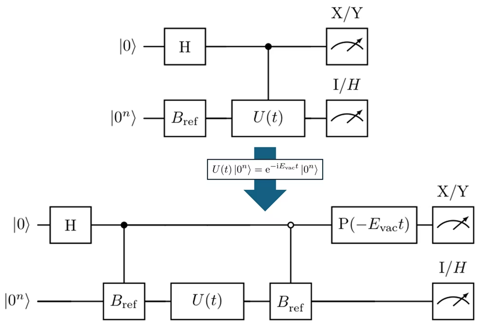
Here, $B_{\rm ref}$ prepares the reference state, $B_{\rm ref}|0^n\rangle = |\psi_{0}\rangle$ .

Instead of first preparing $\frac{1}{\sqrt{2}}(|0\rangle+|1\rangle)|\psi_0\rangle$ and then applying $U(t)$ only on the $|1\rangle$ branch, the circuit directly prepares the two branches as

\begin{equation*} |0\rangle|\psi_0\rangle \quad \text{and} \quad |1\rangle|\psi_d\rangle , \end{equation*}

where

\begin{equation*} |\psi_d\rangle = U(d\Delta t)|\psi_0\rangle . \end{equation*}

The circuit first applies a Hadamard gate to the ancilla and prepares the reference state only on the $|1\rangle$ branch:

\begin{equation*} |0\rangle |0^n\rangle \longrightarrow \frac{|0\rangle |0^n\rangle + |1\rangle B_{\rm ref}|0^n\rangle}{\sqrt{2}} = \frac{|0\rangle |0^n\rangle + |1\rangle |\psi_0\rangle}{\sqrt{2}} . \end{equation*}

Then the uncontrolled time-evolution operator is applied to both branches:

\begin{equation*} \frac{|0\rangle |0^n\rangle + |1\rangle |\psi_0\rangle}{\sqrt{2}} \longrightarrow \frac{|0\rangle U(t)|0^n\rangle + |1\rangle U(t)|\psi_0\rangle}{\sqrt{2}} . \end{equation*}

Since the Hamiltonian preserves the excitation number, we can see that $|0^n\rangle$ is its eigenstate, and thus the evolution operator only accumulates a phase under the Hamiltonian:

\begin{equation*} U(t)|0^n\rangle = e^{-iE_{\rm vac}t}|0^n\rangle . \end{equation*}

Therefore,

\begin{equation*} \frac{|0\rangle U(t)|0^n\rangle + |1\rangle U(t)|\psi_0\rangle}{\sqrt{2}} = \frac{e^{-iE_{\rm vac}t}|0\rangle |0^n\rangle + |1\rangle U(t)|\psi_0\rangle}{\sqrt{2}} . \end{equation*}

Next, $B_{\rm ref}$ is applied only on the $|0\rangle$ branch.

\begin{equation*} \frac{e^{-iE_{\rm vac}t}|0\rangle |\psi_0\rangle + |1\rangle U(t)|\psi_0\rangle}{\sqrt{2}} . \end{equation*}

At this point, the two branches have an extra relative phase. To remove it, we apply the ancilla phase gate

\begin{equation*} P(-E_{\rm vac}t) = \begin{pmatrix} 1 & 0 \\ 0 & e^{-iE_{\rm vac}t} \end{pmatrix}. \end{equation*}

This transforms the state as

\begin{equation*} \frac{e^{-iE_{\rm vac}t}|0\rangle |\psi_0\rangle + |1\rangle U(t)|\psi_0\rangle}{\sqrt{2}} \longrightarrow \frac{e^{-iE_{\rm vac}t}|0\rangle |\psi_0\rangle + e^{-iE_{\rm vac}t}|1\rangle U(t)|\psi_0\rangle}{\sqrt{2}} . \end{equation*}

Thus, up to an irrelevant global phase, we finally prepared

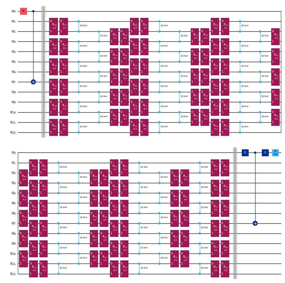
\begin{equation*} |\Phi_{0d}\rangle = \frac{ |0\rangle|\psi_0\rangle + |1\rangle U(t)|\psi_0\rangle }{\sqrt{2}} . \end{equation*}

In the next code block, we implement this control-free circuit.

controlled_extended_swap_test = extended_swap_test

# Reuse the ordering and synthesis rule selected by the comparison above.
evol_gate_optimized = PauliEvolutionGate(
    hamiltonian_for_synthesis,
    time=t,
    synthesis=SuzukiTrotter(order=2, reps=num_trotter_steps),
)

uncontrolled_evolution = QuantumCircuit(num_qubits, name="U_ST2(t)")
uncontrolled_evolution.append(evol_gate_optimized, range(num_qubits))

controlled_state_prep = QuantumCircuit(num_qubits + 1, name="C-Prep")
for q, bit in enumerate(reversed(ref_bitstring)):
    if bit == "1":
        controlled_state_prep.cx(ancilla, system_qubits[q])

vacuum_bitstring = "0" * num_qubits
vacuum_energy = basis_state_expectation_sparse(hamiltonian, "0" * num_qubits)

optimized_extended_swap_test = QuantumCircuit(num_qubits + 1)
optimized_extended_swap_test.h(ancilla)

# Prepare |psi_ref> only on the |1> branch.
optimized_extended_swap_test.compose(controlled_state_prep, inplace=True)
optimized_extended_swap_test.barrier()

# Apply the Trotterized time evolution without control.
optimized_extended_swap_test.compose(
    uncontrolled_evolution,
    qubits=system_qubits,
    inplace=True,
)
optimized_extended_swap_test.barrier()

# Map |0>|0...0> to |0>|psi_ref>, leaving the |1> branch unchanged.
optimized_extended_swap_test.x(ancilla)
optimized_extended_swap_test.compose(controlled_state_prep, inplace=True)
optimized_extended_swap_test.x(ancilla)

# Cancel the known vacuum phase so that the same X/Y observables can be used.
optimized_extended_swap_test.p(-vacuum_energy * t, ancilla)
optimized_extended_swap_test = simple_transpilation(
    optimized_extended_swap_test
)

print(f"Vacuum energy E_vac = {vacuum_energy:.1f}")
display(
    optimized_extended_swap_test.assign_parameters({t: 1.0}).draw(
        "mpl", scale=0.5, fold=26
    )
)

Vacuum energy E_vac = 11.0+0.0j

Output of the previous code cell

Transpilation

Now, we transpile the controlled- and control-free circuits to become executable on the hardware. Let's compare the result of the transpiled circuits.

pass_manager = generate_preset_pass_manager(
    backend=backend,
    optimization_level=3,
)

isa_controlled_extended_swap_test = pass_manager.run(
    controlled_extended_swap_test
)

pass_manager = generate_preset_pass_manager(
    backend=backend, optimization_level=3, routing_method="none"
)
isa_optimized_extended_swap_test = pass_manager.run(
    optimized_extended_swap_test
)

transpilation_result = [
    {
        "label": "abstract controlled U(t)",
        **summarize_circuit(isa_controlled_extended_swap_test),
    },
    {
        "label": "optimized non-controlled U(t)",
        **summarize_circuit(isa_optimized_extended_swap_test),
    },
]

display(pd.DataFrame(transpilation_result))

def filter_qubits_from_layout(layout):
    q_layout = Layout(
        {
            physical: virtual
            for physical, virtual in layout.get_physical_bits().items()
            if virtual._register.name == "q"
        }
    )
    return q_layout

print(
    filter_qubits_from_layout(
        isa_optimized_extended_swap_test.layout.initial_layout
    )
)

isa_observables = [
    op.apply_layout(isa_optimized_extended_swap_test.layout)
    for op in observables
]

label  depth   size  2q gates  2q depth
0       abstract controlled U(t)  15457  23786      4686      4580
1  optimized non-controlled U(t)    261   1716       307        57

Layout({
<Qubit register=(13, "q"), index=0>,
<Qubit register=(13, "q"), index=1>,
<Qubit register=(13, "q"), index=2>,
<Qubit register=(13, "q"), index=3>,
<Qubit register=(13, "q"), index=4>,
<Qubit register=(13, "q"), index=5>,
<Qubit register=(13, "q"), index=6>,
<Qubit register=(13, "q"), index=7>,
<Qubit register=(13, "q"), index=8>,
<Qubit register=(13, "q"), index=9>,
<Qubit register=(13, "q"), index=10>,
<Qubit register=(13, "q"), index=11>,
<Qubit register=(13, "q"), index=12>
})

Step 3: Execute using Qiskit primitives

The next step is to submit the same parameterized circuit for several values of $d$ . For each $d$ , we estimate four expectation values: $X\otimes I$ , $Y\otimes I$ , $X\otimes (H-T)$ , and $Y\otimes (H-T)$ . These four numbers are then combined into the complex first-row elements $\mathcal{S}_{0d}$ and $\mathcal{H}_{0d}$ .

Here, $\mathcal{S}_{00}=1$ and $\mathcal{H}_{00}=\langle\psi_{0}|(H-T)|\psi_{0}\rangle=\langle\psi_{0}|H|\psi_{0}\rangle-\tau$ can be classically calculated since $\lvert\psi_0\rangle$ is sparse, so we skip the $d=0$ case.

pub_list = []
d_values = list(range(1, krylov_dim))

# Exact local statevector estimator.
estimator = StatevectorEstimator()

# We use the circuit before the transpilation for the local simulator,
# but we will use the transpiled circuit for the real backend.
for d in d_values:
    parameter_values = [d * dt]

    for ob in observables:
        pub_list.append(
            (
                optimized_extended_swap_test,
                ob,
                parameter_values,
            )
        )

job = estimator.run(pub_list)

# Local PrimitiveJob does not provide Runtime-style job inputs,
# so preserve the inputs directly.
inputs = pub_list
result = job.result()

print(f"Number of Krylov basis states: r = {len(d_values)}")
print(f"Number of PUBs: {len(pub_list)}")
print(f"Each d uses observables: {observable_labels}")

Number of Krylov basis states: r = 9
Number of PUBs: 36
Each d uses observables: ['Re S_0d', 'Im S_0d', 'Re shifted H_0d', 'Im shifted H_0d']

Step 4: Post-process and return result in desired classical format

After estimating the projected matrices, we regularize and solve the GEVP

\begin{equation*} \mathcal{H}\mathbf{c} = E\mathcal{S}\mathbf{c}. \end{equation*}

The smallest generalized eigenvalue gives the KQD estimate of the ground-state energy.

h_shifted_row_est = np.zeros(krylov_dim, dtype=complex)
s_row_est = np.zeros(krylov_dim, dtype=complex)

h_shifted_row_est[0] = ref_energy - shift_tau
s_row_est[0] = 1.0

for idx, (pub_input, pub_result) in enumerate(zip(inputs, result)):
    d_index, obs_index = divmod(idx, len(observables))
    ev = np.asarray(pub_result.data.evs).reshape(-1)[0]
    std = np.asarray(pub_result.data.stds).reshape(-1)[0]

    if obs_index == 0:
        s_row_est[d_index + 1] = ev
    elif obs_index == 1:
        s_row_est[d_index + 1] += 1j * ev
    elif obs_index == 2:
        h_shifted_row_est[d_index + 1] = ev
    elif obs_index == 3:
        h_shifted_row_est[d_index + 1] += 1j * ev

# H_0d = shifted_H_0d + tau * S_0d.
h_row_est = h_shifted_row_est + shift_tau * s_row_est

h_matrix_est = la.toeplitz(h_row_est.conj(), h_row_est)
s_matrix_est = la.toeplitz(s_row_est.conj(), s_row_est)

s_eigvals = la.eigvalsh(0.5 * (s_matrix_est + s_matrix_est.conj().T))
positive_s_eigvals = s_eigvals[s_eigvals > 1e-12]
s_condition_number = (
    positive_s_eigvals[-1] / positive_s_eigvals[0]
    if len(positive_s_eigvals) > 0
    else np.inf
)

with np.printoptions(precision=3, suppress=True):
    print("Estimated first row of S:")
    print(s_row_est)
    print()
    print("Estimated first row of H:")
    print(h_row_est)
    print()
    print("Eigenvalues of the estimated overlap matrix S:")
    print(s_eigvals)
    print(f"Condition number above 1e-12: {s_condition_number:.3e}")
    print()

Estimated first row of S:
[ 1.   +0.j     0.758-0.596j  0.203-0.836j -0.291-0.636j -0.444-0.229j
 -0.276+0.053j -0.044+0.051j  0.006-0.121j -0.155-0.218j -0.345-0.101j]

Estimated first row of H:
[ 7.   +0.j     4.842-4.76j   0.044-6.185j -3.791-3.653j -4.137+0.39j
 -1.495+2.654j  1.331+1.777j  1.85 -0.763j -0.032-2.278j -2.222-1.372j]

Eigenvalues of the estimated overlap matrix S:
[-0.     0.     0.     0.     0.     0.     0.01   0.355  3.526  6.109]
Condition number above 1e-12: 1.904e+12

Now we solve the generalized eigenvalue problem using the matrices reconstructed from the circuit estimates. In an ideal statevector calculation with exact real-time evolution, this should reproduce the exact projected result. In practice, deviations can come from Trotterization, sampling error, and numerical instability of the overlap matrix.

We observe how the energy converges as we increase the dimension of the Krylov subspace.

exact_evals = diagonalize_single_1_subspace(hamiltonian)
exact_ground = min(exact_evals)
print("exact ground state energy:  ", exact_ground)

threshold = 1e-12
energy_convergence = []

for r in range(1, krylov_dim + 1):
    energy_est_kqd, coeffs_est, retained_est = solve_thresholded_gevp(
        h_matrix_est[:r, :r],
        s_matrix_est[:r, :r],
        threshold=threshold,
    )
    energy_convergence.append(energy_est_kqd)
    print(
        f"Krylov ground state energy (dim={r}, retained={retained_est}): ",
        energy_est_kqd,
    )

exact ground state energy:   3.136296694843727
Krylov ground state energy (dim=1, retained=1):  7.0
Krylov ground state energy (dim=2, retained=2):  4.184510657551266
Krylov ground state energy (dim=3, retained=3):  3.5539074630394136
Krylov ground state energy (dim=4, retained=4):  3.3366270761341044
Krylov ground state energy (dim=5, retained=5):  3.252017453225087
Krylov ground state energy (dim=6, retained=6):  3.2300275138879186
Krylov ground state energy (dim=7, retained=7):  3.2299154099085685
Krylov ground state energy (dim=8, retained=7):  3.2298063744216776
Krylov ground state energy (dim=9, retained=7):  3.2296778282872456
Krylov ground state energy (dim=10, retained=8):  3.223647515867734

def plot_energy_convergence(energy_convergence, exact_ground, krylov_dim):
    fig, ax = plt.subplots(figsize=(7, 4.5))

    ax.plot(
        range(1, krylov_dim + 1),
        energy_convergence,
        marker="o",
        label="KQD estimate",
    )

    ax.axhline(
        exact_ground,
        linestyle="--",
        label=f"Exact ground energy = {exact_ground:.6f}",
    )

    ax.set_xlabel("Krylov dimension")
    ax.set_ylabel("Ground-state energy")
    ax.grid(True, alpha=0.3)
    ax.legend()
    plt.tight_layout()
    plt.show()

plot_energy_convergence(energy_convergence, exact_ground, krylov_dim)

Output of the previous code cell

Large-scale hardware example

The previous section used a 12-qubit model so that the statevector simulation could be used as a diagnostic. We now scale the same KQD workflow to a 30-qubit Heisenberg chain and prepare the workload for execution on IBM Quantum hardware.

Steps 1-4 compressed into a single code block

Here we now put all of these details together into a singular workflow at a larger scale, which is then run on our real quantum hardware. In this section, we apply realistic error-mitigation settings to improve the reliability of the results. Since the matrix elements corresponding to different values of $d$ can be evaluated in parallel, we use Batch mode to execute them efficiently.

# -------------------------Step 1-------------------------

# Map the classical problem to quantum circuits and observables.
# Problem and KQD parameters.
large_num_qubits = 30
large_krylov_dim = 7
large_num_trotter_steps = 3
large_dt = np.pi / (3 * (large_num_qubits - 1))
large_t = Parameter("t_large")

# Use a single excitation near the center of the chain.
large_excitation_qubit = large_num_qubits // 2
large_ref_label = ["0"] * large_num_qubits
large_ref_label[large_num_qubits - 1 - large_excitation_qubit] = "1"
large_ref_bitstring = "".join(large_ref_label)

# Use the ordering and product formula selected in the preceding section.
large_hamiltonian = make_heisenberg_hamiltonian_ordered(
    large_num_qubits,
    ordering="even-odd edge-grouped",
    coupling=1.0,
)
large_ref_energy = float(
    np.real(
        basis_state_expectation_sparse(large_hamiltonian, large_ref_bitstring)
    )
)
large_vacuum_energy = float(
    np.real(
        basis_state_expectation_sparse(
            large_hamiltonian, "0" * large_num_qubits
        )
    )
)

large_evolution_gate = PauliEvolutionGate(
    large_hamiltonian,
    time=large_t,
    synthesis=SuzukiTrotter(order=2, reps=large_num_trotter_steps),
)
large_uncontrolled_evolution = QuantumCircuit(
    large_num_qubits,
    name="U_ST2_large(t)",
)
large_uncontrolled_evolution.append(
    large_evolution_gate,
    range(large_num_qubits),
)

# Build the control-free extended-swap-test circuit.
large_ancilla = 0
large_system_qubits = list(range(1, large_num_qubits + 1))

large_controlled_state_prep = QuantumCircuit(
    large_num_qubits + 1,
    name="C-Prep-large",
)
large_controlled_state_prep.cx(
    large_ancilla,
    large_system_qubits[large_excitation_qubit],
)

large_extended_swap_test = QuantumCircuit(large_num_qubits + 1)
large_extended_swap_test.h(large_ancilla)
large_extended_swap_test.compose(large_controlled_state_prep, inplace=True)
large_extended_swap_test.compose(
    large_uncontrolled_evolution,
    qubits=large_system_qubits,
    inplace=True,
)
large_extended_swap_test.x(large_ancilla)
large_extended_swap_test.compose(
    large_controlled_state_prep.inverse(),
    inplace=True,
)
large_extended_swap_test.x(large_ancilla)
large_extended_swap_test.p(
    -large_vacuum_energy * large_t,
    large_ancilla,
)

# Reuse the Hamiltonian-shifting construction from the preceding section.
(
    large_obs_x_shifted_hamiltonian,
    large_obs_y_shifted_hamiltonian,
    large_shift_tau,
) = make_reduced_heisenberg_observables(large_ref_bitstring)

large_observables = [
    SparsePauliOp("I" * large_num_qubits + "X"),
    SparsePauliOp("I" * large_num_qubits + "Y"),
    large_obs_x_shifted_hamiltonian,
    large_obs_y_shifted_hamiltonian,
]
large_observable_labels = [
    "Re S_0d",
    "Im S_0d",
    "Re shifted H_0d",
    "Im shifted H_0d",
]

# -------------------------Step 2-------------------------

# Optimize the problem for quantum execution.
# Select a real backend and transpile the parameterized circuit to ISA form.
large_backend = service.backend("ibm_boston")
large_pass_manager = generate_preset_pass_manager(
    backend=large_backend, optimization_level=3, routing_method="none"
)
large_isa_circuit = large_pass_manager.run(large_extended_swap_test)
large_isa_observables = [
    observable.apply_layout(large_isa_circuit.layout)
    for observable in large_observables
]

large_two_qubit_gate_count = sum(
    instruction.operation.num_qubits == 2
    for instruction in large_isa_circuit.data
)

print(f"Backend: {large_backend.name}")
print(f"System qubits: {large_num_qubits}")
print(f"Total circuit qubits: {large_isa_circuit.num_qubits}")
print(f"Krylov dimension: {large_krylov_dim}")
print(f"Time step: {large_dt:.6f}")
print(f"Shift tau: {large_shift_tau}")
print(f"ISA circuit depth: {large_isa_circuit.depth()}")
print(f"ISA two-qubit gates: {large_two_qubit_gate_count}")
print(
    f"ISA two-qubit depth: {large_isa_circuit.depth(lambda x: x[0].num_qubits == 2)}"
)

# -------------------------Step 3-------------------------

# Execute on quantum hardware with Qiskit Runtime primitives.
# Submit one job per d, with all four observables in that job.
large_d_values = list(range(1, large_krylov_dim))
retrieve_batch_id = None
large_jobs = []

if retrieve_batch_id is None:
    large_estimator_options = {
        "default_shots": 8192,
        "dynamical_decoupling": {
            "enable": True,
            "sequence_type": "XpXm",
        },
        "resilience": {
            "measure_mitigation": True,
            "measure_noise_learning": {
                "num_randomizations": 32,
                "shots_per_randomization": 256,
            },
            "layer_noise_learning": {
                "max_layers_to_learn": 4,
                "layer_pair_depths": [0, 1, 2, 4, 16, 32],
                "num_randomizations": 32,
                "shots_per_randomization": 128,
            },
            "zne_mitigation": True,
            "zne": {
                "amplifier": "pea",
                "noise_factors": [1.0, 1.5, 2.0],
                "extrapolator": ("exponential", "linear"),
            },
        },
        "twirling": {
            "enable_gates": True,
            "enable_measure": True,
            "num_randomizations": 32,
            "shots_per_randomization": 256,
            "strategy": "active-accum",
        },
    }

    with Batch(backend=large_backend) as large_batch:
        large_batch_id = large_batch.session_id
        large_estimator = EstimatorV2(
            mode=large_batch,
            options=large_estimator_options,
        )
        # Krylov quantum diagonalization of lattice Hamiltonians -> TUT_KQDOLH.
        large_estimator.options.environment.job_tags = ["TUT_KQDOLH"]

        for d in large_d_values:
            parameter_values = [d * large_dt]
            pubs_for_d = [
                (large_isa_circuit, observable, parameter_values)
                for observable in large_isa_observables
            ]
            job = large_estimator.run(pubs_for_d)
            large_jobs.append(job)
            print(
                f"Submitted d={d}: job_id={job.job_id()}, "
                f"PUBs={len(pubs_for_d)}"
            )

    print(f"Batch ID: {large_batch_id}")
else:
    large_batch_id = retrieve_batch_id
    large_jobs = service.jobs(
        session_id=large_batch_id,
        limit=None,
        descending=False,
    )

large_job_ids_by_d = {
    d: job.job_id() for d, job in zip(large_d_values, large_jobs)
}
print(f"Job IDs by d: {large_job_ids_by_d}")

# -------------------------Step 4-------------------------

# Post-process the quantum results and solve the classical GEVP.
# Reconstruct the first rows of S and the shifted Hamiltonian matrix.
large_s_row_est = np.zeros(large_krylov_dim, dtype=complex)
large_h_shifted_row_est = np.zeros(large_krylov_dim, dtype=complex)
large_s_row_est[0] = 1.0
large_h_shifted_row_est[0] = large_ref_energy - large_shift_tau

for d, job in zip(large_d_values, large_jobs):
    job_result = job.result()

    if len(job_result) != len(large_observables):
        raise RuntimeError(
            f"Expected {len(large_observables)} PUB results for d={d}, "
            f"but received {len(job_result)}."
        )

    expectation_values = [
        np.asarray(pub_result.data.evs).reshape(-1)[0]
        for pub_result in job_result
    ]

    large_s_row_est[d] = expectation_values[0] + 1j * expectation_values[1]
    large_h_shifted_row_est[d] = (
        expectation_values[2] + 1j * expectation_values[3]
    )

# H_0d = shifted_H_0d + tau * S_0d.
large_h_row_est = large_h_shifted_row_est + large_shift_tau * large_s_row_est

large_s_matrix_est = la.toeplitz(
    large_s_row_est.conj(),
    large_s_row_est,
)
large_h_matrix_est = la.toeplitz(
    large_h_row_est.conj(),
    large_h_row_est,
)

large_exact_gnd = min(diagonalize_single_1_subspace(large_hamiltonian))

large_energy_convergence = []

with np.printoptions(precision=5, suppress=True):
    print("Estimated first row of S:")
    print(large_s_row_est)
    print("Estimated first row of H:")
    print(large_h_row_est)
    print("exact ground state energy:  ", large_exact_gnd)

    for r in range(1, large_krylov_dim + 1):
        energy_est_kqd, coeffs_est, retained_est = solve_thresholded_gevp(
            large_h_matrix_est[:r, :r],
            large_s_matrix_est[:r, :r],
            threshold=5e-2,
        )
        large_energy_convergence.append(energy_est_kqd)
        print(
            f"Krylov ground state energy (dim={r}, retained={retained_est}): ",
            energy_est_kqd,
        )

plot_energy_convergence(
    large_energy_convergence, large_exact_gnd, large_krylov_dim
)

Backend: ibm_boston
System qubits: 30
Total circuit qubits: 156
Krylov dimension: 7
Time step: 0.036110
Shift tau: 25.0
ISA circuit depth: 219
ISA two-qubit gates: 728
ISA two-qubit depth: 52
Job IDs by d: {1: 'd9fl4p4jeosc73fk4dg0', 2: 'd9fl4pineu4c739poecg', 3: 'd9fl4q2neu4c739poedg', 4: 'd9fl4qhhtsac739fjgn0', 5: 'd9fl4r4jeosc73fk4dhg', 6: 'd9fl4rkjeosc73fk4dj0'}
Estimated first row of S:
[ 1.     +0.j       0.42055-0.65466j -0.17883-0.73125j -0.64523-0.31601j
 -0.70781+0.55574j -0.02467+0.70525j  0.59301+0.55602j]
Estimated first row of H:
[ 25.      +0.j       10.3419 -16.5586j   -5.017  -18.03933j
 -16.44797 -6.98173j -17.17081+14.84502j   0.62722+17.81196j
  15.68886+12.74875j]
exact ground state energy:   21.021912418526902
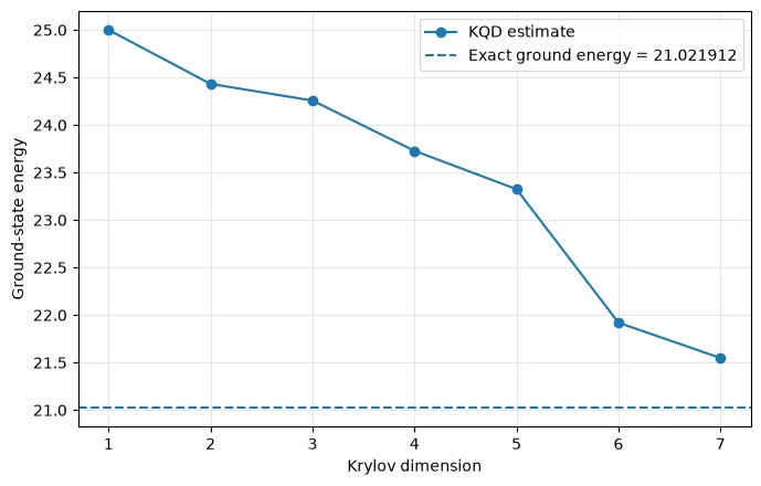
Krylov ground state energy (dim=1, retained=1):  25.0
Krylov ground state energy (dim=2, retained=2):  24.432409110686205
Krylov ground state energy (dim=3, retained=3):  24.256856893278556
Krylov ground state energy (dim=4, retained=4):  23.727409826799715
Krylov ground state energy (dim=5, retained=4):  23.324720470780864
Krylov ground state energy (dim=6, retained=5):  21.91957579005085
Krylov ground state energy (dim=7, retained=5):  21.548331214122644

Output of the previous code cell

Appendix: The Hamiltonian-function (spectral-filter) viewpoint

The main workflow presented KQD operationally: build a Krylov basis from real-time-evolved states, estimate the projected matrices $\mathcal{H}$ and $\mathcal{S}$ , and solve the GEVP. This appendix revisits the same computation from a complementary angle that explains why KQD works: the Hamiltonian-function, or spectral-filter, viewpoint [3], [5]. It reuses the 12-qubit model, time step $\Delta t$ , and the Krylov solution already obtained above; no new circuit execution is required.

The reference state as an energy distribution

Let the Hamiltonian have the eigendecomposition

\begin{equation*} H=\sum_{m} E_m\,|E_m\rangle\!\langle E_m|, \qquad E_0\le E_1\le\cdots, \end{equation*}

with energy eigenstates $|E_m\rangle$ . Any reference state can be expanded in this eigenbasis,

\begin{equation*} |\psi_{0}\rangle=\sum_m a_m\,|E_m\rangle, \qquad a_m=\langle E_m|\psi_{0}\rangle, \end{equation*}

so it carries a spectral weight $p_m=|a_m|^2$ at each energy $E_m$ . The reference energy is the mean of this distribution, $\langle H\rangle_{0}=\sum_m p_m E_m$ .

The eigendecomposition of a general $n$ -qubit Hamiltonian is exponentially costly, so this picture is only a diagnostic, which is not part of the algorithm. Here, however, we can compute it cheaply for the same $n=12$ problem: the Heisenberg Hamiltonian conserves the total excitation number, and the reference $|000001000000\rangle$ carries a single excitation, so its entire spectral content lives in the single-excitation subspace whose dimension grows only linearly with $n$ . We therefore reuse the exact single-excitation block (already used above as a benchmark) and read off the reference distribution $\{(E_m, p_m)\}$ inside that subspace.

# Exact single-excitation-subspace decomposition of the reference state.
# This reuses make_heisenberg_hamiltonian / _basis_state_transition_amplitude_sparse
# and the n=12 `hamiltonian` and `ref_bitstring` defined in the small-scale example.
single_excitation_states = [1 << k for k in range(num_qubits)]

h_single = np.array(
    [
        [
            _basis_state_transition_amplitude_sparse(hamiltonian, bra, ket)
            for ket in single_excitation_states
        ]
        for bra in single_excitation_states
    ]
)
h_single = 0.5 * (h_single + h_single.conj().T)

subspace_evals, subspace_evecs = la.eigh(h_single)
subspace_evals = np.real(subspace_evals)

# Reference-state coordinates inside the single-excitation subspace.
ref_position = single_excitation_states.index(int(ref_bitstring, 2))
ref_in_subspace = np.zeros(num_qubits, dtype=complex)
ref_in_subspace[ref_position] = 1.0

# Amplitudes and spectral weights of the reference in the energy eigenbasis.
ref_eigen_amplitudes = subspace_evecs.conj().T @ ref_in_subspace
ref_spectral_weights = np.abs(ref_eigen_amplitudes) ** 2

print(f"Single-excitation subspace dimension: {num_qubits}")
print(f"Subspace ground-state energy:         {subspace_evals[0]:.6f}")
print(
    f"Reference energy (sum p_m E_m):       {np.sum(ref_spectral_weights * subspace_evals):.6f}"
)
print(f"Reference weight on subspace ground:  {ref_spectral_weights[0]:.6f}")

Single-excitation subspace dimension: 12
Subspace ground-state energy:         3.136297
Reference energy (sum p_m E_m):       7.000000
Reference weight on subspace ground:  0.163827

KQD learns a filter that reshapes this distribution

A Hamiltonian function $f(H)$ is defined through spectral calculus,

\begin{equation*} f(H)=\sum_m f(E_m)\,|E_m\rangle\!\langle E_m|, \end{equation*}

or in other words, a weighted sum of eigenprojectors. Applying it to the reference reshapes each spectral amplitude, $a_m \to a_m f(E_m)$ :

\begin{equation*} f(H)\,|\psi_{0}\rangle=\sum_m a_m\,f(E_m)\,|E_m\rangle . \end{equation*}

If $f$ were sharply peaked at the lowest energy ( $f(E_0)=1$ and $f(E_m)\approx 0$ otherwise) then $f(H)$ would act as a ground-state projector, and the normalized output would be (close to) the ground state. Therefore, a good low-pass spectral filter in energy is exactly what we want.

KQD does not prescribe $f$ in advance. Instead it expands the filter in the real-time-evolution basis,

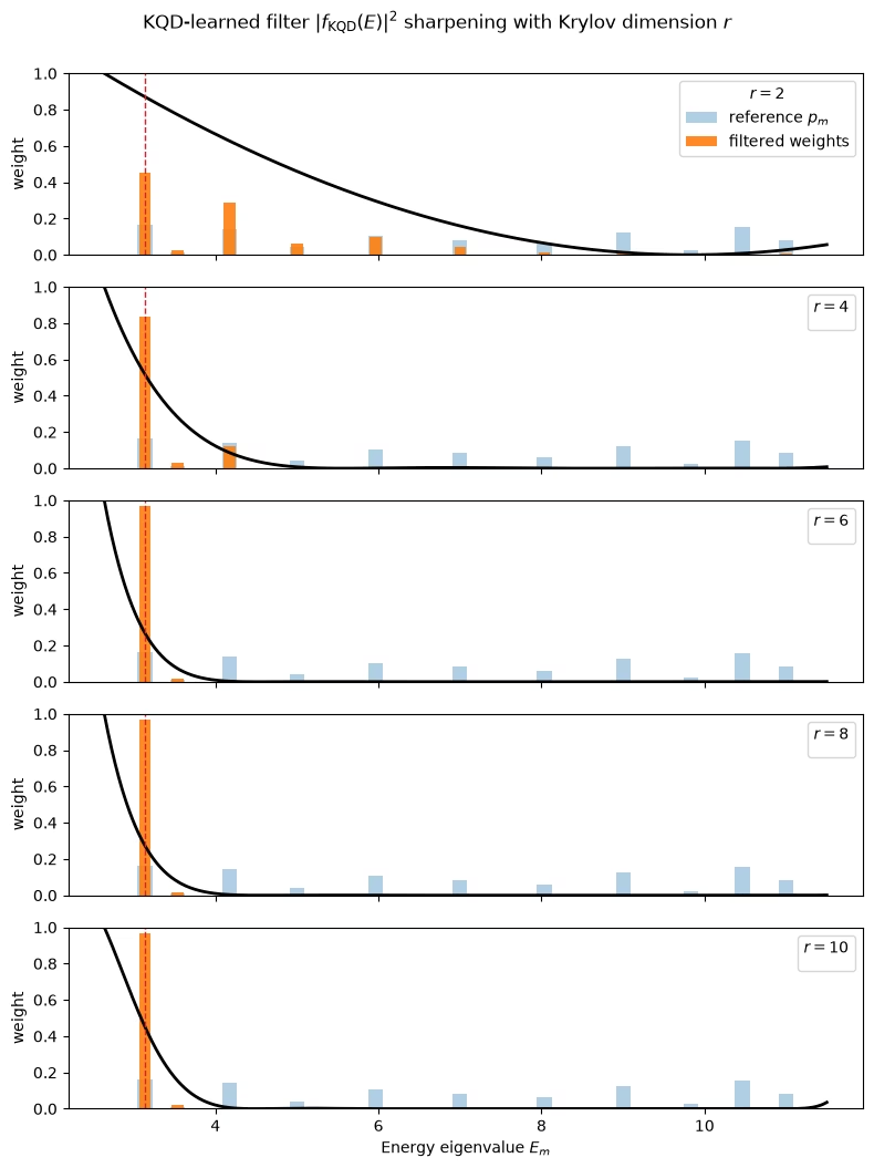
\begin{equation*} f_{\rm KQD}(E)=\sum_{\ell=0}^{r-1} c_\ell\, e^{-i\ell\Delta t E}, \end{equation*}

a trigonometric function of the energy whose coefficients $\{c_\ell\}$ are precisely the GEVP eigenvector solved for above. Minimizing the Rayleigh quotient $\mathbf{c}^\dagger\mathcal{H}\mathbf{c}/\mathbf{c}^\dagger\mathcal{S}\mathbf{c}$ is therefore the same as learning the filter that best suppresses the excited-state weight of the reference. Larger Krylov dimension $r$ gives the filter more degrees of freedom and a sharper peak at the ground-state energy.

The helper below evaluates this learned filter on an energy axis; we then apply it to the reference distribution obtained above.

def trigonometric_krylov_filter(
    coeffs: np.ndarray,
    energies: np.ndarray,
    time_step: float,
) -> np.ndarray:
    """Evaluate the learned Krylov filter f(E) = sum_l c_l exp(-i l dt E)."""
    values = np.zeros_like(energies, dtype=complex)
    for ell, coeff in enumerate(coeffs):
        values += coeff * np.exp(-1j * ell * time_step * energies)
    return values

def filtered_spectral_weights(
    weights: np.ndarray,
    filter_values: np.ndarray,
) -> np.ndarray:
    """Reshape spectral weights by |f(E)|^2 and renormalize."""
    reshaped = weights * np.abs(filter_values) ** 2
    return reshaped / np.sum(reshaped)

# Recover the KQD coefficients from the already-estimated projected matrices.
# The shift only moves H by tau * S, so it does not change the GEVP eigenvector;
# we solve at the full Krylov dimension used in the small-scale example.
_, kqd_coeffs, _ = solve_thresholded_gevp(
    h_matrix_est,
    s_matrix_est,
    threshold=1e-12,
)

filter_on_spectrum = trigonometric_krylov_filter(
    kqd_coeffs, subspace_evals, dt
)
filtered_weights = filtered_spectral_weights(
    ref_spectral_weights, filter_on_spectrum
)

print(f"Ground-state overlap  (reference): {ref_spectral_weights[0]:.4f}")
print(f"Ground-state overlap  (filtered):  {filtered_weights[0]:.4f}")
print(
    f"Mean energy           (reference): {np.sum(ref_spectral_weights * subspace_evals):.6f}"
)
print(
    f"Mean energy           (filtered):  {np.sum(filtered_weights * subspace_evals):.6f}"
)

Ground-state overlap  (reference): 0.1638
Ground-state overlap  (filtered):  0.9638
Mean energy           (reference): 7.000000
Mean energy           (filtered):  3.164503

Visualize the filter and its flexibility

We first show the learned filter at the full Krylov dimension used above, then track how it sharpens as the dimension $r$ grows.

The bars show the reference spectral weights $p_m$ (before) and the filtered weights $p_m|f_{\rm KQD}(E_m)|^2$ (after), together with the learned filter intensity $|f_{\rm KQD}(E)|^2$ on a continuous energy axis. The filter concentrates the weight onto the lowest energy of the single-excitation subspace — the same energy that the KQD estimate converged to in the small-scale example. Note that this is the ground state within the single-excitation sector, which is the relevant target for this excitation-conserving reference state, not the global ground state.

fig, ax = plt.subplots(figsize=(8, 4))

visible = (ref_spectral_weights > 1e-4) | (filtered_weights > 1e-4)
ax.bar(
    subspace_evals[visible],
    ref_spectral_weights[visible],
    width=0.18,
    alpha=0.45,
    label="reference $p_m$",
)
ax.bar(
    subspace_evals[visible],
    filtered_weights[visible],
    width=0.14,
    alpha=0.9,
    label=r"filtered $p_m\,|f_{\rm KQD}(E_m)|^2$",
)

energy_grid = np.linspace(
    subspace_evals.min() - 0.5, subspace_evals.max() + 0.5, 800
)
filter_intensity = (
    np.abs(trigonometric_krylov_filter(kqd_coeffs, energy_grid, dt)) ** 2
)
filter_intensity /= filter_intensity.max()
ax.plot(
    energy_grid,
    filter_intensity,
    color="k",
    linewidth=2,
    label=r"$|f_{\rm KQD}(E)|^2$ (normalized)",
)

ax.axvline(
    subspace_evals[0],
    color="C3",
    linestyle="--",
    linewidth=1,
    label="subspace ground energy",
)
ax.set_xlabel("Energy eigenvalue $E_m$")
ax.set_ylabel("Spectral weight")
ax.set_ylim(0, 1)
ax.legend(loc="upper right")
plt.tight_layout()
plt.show()

Output of the previous code cell

Increasing the Krylov dimension: flexibility of the learned function

Recall that the learned filter is a trigonometric polynomial in the energy with $r$ coefficients,

\begin{equation*} f_{\rm KQD}(E)=\sum_{\ell=0}^{r-1} c_\ell\, e^{-i\ell\Delta t E}. \end{equation*}

The Krylov dimension $r$ is exactly the number of free coefficients, so it controls the flexibility of the function. A small $r$ can only produce a broad, gently varying filter that leaks weight into low-lying excited states; when $r$ increases, the filter can form a narrower peak at the target energy and suppress the remaining excited-state weight more aggressively. This is the spectral-filter counterpart of the energy convergence observed in the small-scale example: as $r$ grows, the filtered distribution collapses onto the subspace ground state and the estimated energy decreases toward it.

We reuse the projected matrices already estimated above and simply solve the GEVP at each leading $r\times r$ block, then evaluate and plot the corresponding filter.

# Sweep the Krylov dimension using the leading r x r blocks of the estimated matrices.
sweep_dims = [r for r in (2, 4, 6, 8, krylov_dim) if r <= krylov_dim]
sweep_dims = sorted(set(sweep_dims))

energy_grid = np.linspace(
    subspace_evals.min() - 0.5, subspace_evals.max() + 0.5, 800
)

sweep_cases = []
print(" r    retained    ground overlap    filtered energy")
print("--    --------    --------------    ---------------")
for r in sweep_dims:
    _, coeffs_r, retained_r = solve_thresholded_gevp(
        h_matrix_est[:r, :r],
        s_matrix_est[:r, :r],
        threshold=1e-12,
    )
    filter_on_spectrum_r = trigonometric_krylov_filter(
        coeffs_r, subspace_evals, dt
    )
    filtered_weights_r = filtered_spectral_weights(
        ref_spectral_weights, filter_on_spectrum_r
    )
    filtered_energy_r = float(np.sum(filtered_weights_r * subspace_evals))

    sweep_cases.append((r, coeffs_r, filtered_weights_r))
    print(
        f"{r:2d}    {retained_r:8d}    {filtered_weights_r[0]:14.4f}    {filtered_energy_r:15.6f}"
    )

print(f"\nSubspace ground-state energy (target): {subspace_evals[0]:.6f}")

# One panel per Krylov dimension: filtered spectrum (bars) + filter intensity (curve).
fig, axes = plt.subplots(
    len(sweep_cases),
    1,
    figsize=(8, 2.1 * len(sweep_cases)),
    sharex=True,
)
axes = np.atleast_1d(axes)

for idx, (ax, (r, coeffs_r, filtered_weights_r)) in enumerate(
    zip(axes, sweep_cases)
):
    visible = (ref_spectral_weights > 1e-4) | (filtered_weights_r > 1e-4)
    ax.bar(
        subspace_evals[visible],
        ref_spectral_weights[visible],
        width=0.18,
        alpha=0.35,
        color="C0",
        label="reference $p_m$" if idx == 0 else None,
    )
    ax.bar(
        subspace_evals[visible],
        filtered_weights_r[visible],
        width=0.14,
        alpha=0.9,
        color="C1",
        label="filtered weights" if idx == 0 else None,
    )

    filter_intensity_r = (
        np.abs(trigonometric_krylov_filter(coeffs_r, energy_grid, dt)) ** 2
    )
    filter_intensity_r /= filter_intensity_r.max()
    ax.plot(energy_grid, filter_intensity_r, color="k", linewidth=2)

    ax.axvline(subspace_evals[0], color="C3", linestyle="--", linewidth=1)
    ax.set_ylim(0, 1)
    ax.set_ylabel("weight")
    ax.legend(loc="upper right", title=f"$r={r}$")

axes[-1].set_xlabel("Energy eigenvalue $E_m$")
fig.suptitle(
    r"KQD-learned filter $|f_{\rm KQD}(E)|^2$ sharpening with Krylov dimension $r$",
    y=1.0,
)
fig.tight_layout()
plt.show()

r    retained    ground overlap    filtered energy
--    --------    --------------    ---------------
 2           2            0.4549           4.184510
 4           4            0.8373           3.310168
 6           6            0.9706           3.158100
 8           7            0.9701           3.158725
10           8            0.9638           3.164503

Subspace ground-state energy (target): 3.136297

Output of the previous code cell

Next steps

If you found this work interesting, you might be interested in the following material:

Recommendations

References

[1] E. N. Epperly, L. Lin, and Y. Nakatsukasa, A theory of quantum subspace diagonalization, SIAM Journal on Matrix Analysis and Applications 43, 1263-1290 (2022).

[2] N. Yoshioka, M. Amico, W. Kirby, et al., Diagonalization of large many-body Hamiltonians on a quantum processor, arXiv:2407.14431 (2024).

[3] R. M. Parrish and P. L. McMahon, Quantum filter diagonalization: quantum eigendecomposition without full quantum phase estimation, Physical Review Letters 122, 230401 (2019).

[4] G. Lee, S. Choi, J. Huh, and A. F. Izmaylov, Efficient strategies for reducing sampling error in quantum Krylov subspace diagonalization, Digital Discovery 4, 954-969 (2025).

[5] G. Lee, M. Kang, J. Hong, S. Fomichev and J. Huh, Filtered Quantum Phase Estimation, arXiv:2510.04294 (2025).

Learning outcomes​

Prerequisites​

Background​

Requirements​

Setup​

Small-scale simulator example​

Step 1: Map classical inputs to a quantum problem​

Hamiltonian and reference state​

Set the parameters for the algorithm​

Build circuit​

Reference state​

Time evolution​

Extended swap test circuit [3]​

Observables​

Step 2: Optimize problem for quantum hardware execution​

Compare Hamiltonian term ordering​

Compare product-formula synthesis​

Remove the controlled time-evolution gate​

Transpilation​

Step 3: Execute using Qiskit primitives​

Step 4: Post-process and return result in desired classical format​

Large-scale hardware example​

Steps 1-4 compressed into a single code block​

Appendix: The Hamiltonian-function (spectral-filter) viewpoint​

The reference state as an energy distribution​

KQD learns a filter that reshapes this distribution​

Visualize the filter and its flexibility​

Increasing the Krylov dimension: flexibility of the learned function​

Next steps​

References​

Learning outcomes

Prerequisites

Background

Requirements

Setup

Small-scale simulator example

Step 1: Map classical inputs to a quantum problem

Hamiltonian and reference state

Set the parameters for the algorithm

Build circuit

Reference state

Time evolution

Extended swap test circuit [3]

Observables

Step 2: Optimize problem for quantum hardware execution

Compare Hamiltonian term ordering

Compare product-formula synthesis

Remove the controlled time-evolution gate

Transpilation

Step 3: Execute using Qiskit primitives

Step 4: Post-process and return result in desired classical format

Large-scale hardware example

Steps 1-4 compressed into a single code block

Appendix: The Hamiltonian-function (spectral-filter) viewpoint

The reference state as an energy distribution

KQD learns a filter that reshapes this distribution

Visualize the filter and its flexibility

Increasing the Krylov dimension: flexibility of the learned function

Next steps

References