Pooled sample-based quantum diagonalization of a nuclear Hamiltonian
Usage estimate: 2.5 minutes on a Heron processor (NOTE: This is an estimate only. Your runtime might vary.)
This notebook presents the Python implementation. The Fortran implementation is in the Fortran companion directory of this documentation repository. The Python version adds a self-consistent configuration-recovery step, which the Fortran driver does not perform.
Learning outcomes
- Learn how a nuclear shell-model Hamiltonian, tabulated in a -coupled basis of orbitals, becomes a qubit Hamiltonian in the -scheme, where one qubit is one single-particle state.
- Build a fixed, non-variational excitation ansatz whose angles come from second-order perturbation theory, so there is no classical optimization loop.
- Compare qubit and fermionic excitations and measure how the choice affects the ensemble’s two-qubit depth.
- Run self-consistent configuration recovery with
qiskit-addon-sqdwhen the conserved quantities are nucleon numbers, , and parity rather than electron numbers and spin. - Apply one workflow from a 24-qubit problem you can check exactly to a 40-qubit problem with nearly two million basis states, beyond this tutorial's exact-diagonalization capacity.
Prerequisites
Before starting, review the following topics:
- Sample-based quantum diagonalization and the SQD addon API reference.
- Sample-based quantum diagonalization of a chemistry Hamiltonian, the electronic-structure counterpart of this tutorial.
- Transpile against a backend target and Introduction to primitives.
- Second quantization and the Jordan-Wigner mapping.
Background
The nuclear shell model treats a nucleus as a few valence nucleons moving in a small set of single-particle orbitals above an inert core, interacting through an empirical two-body force fitted to measured spectra. It is widely used in low-energy nuclear structure. Its computational cost is combinatorial: the basis is every way of distributing the valence protons and neutrons over the available states, and this growth limits the model spaces accessible to exact diagonalization.
Pooled sample-based quantum diagonalization (pooled SQD) [1] splits that problem in two. A quantum circuit is used only to propose which basis states matter. It is measured in the computational basis, and each measured bitstring names one Slater determinant. The Hamiltonian is then built and diagonalized classically in the span of those determinants. Because the classical step is an exact diagonalization inside a subspace, it returns a variational upper bound on the true ground-state energy, and the bound can only fall as determinants are added.
This division of work makes the method noise-tolerant, with an important limitation. Noise changes which determinants the circuit proposes. It does not enter the classical Hamiltonian, so it cannot move the eigenvalue of a given subspace: a shot that violates a conserved quantity is discarded or repaired, and a shot that survives is a legitimate basis vector however it was produced. Noise therefore costs you subspace quality, not correctness, and the number you report is an upper bound either way.
Nuclear structure provides several exact quantum numbers for filtering samples. A physical determinant must carry the right number of valence protons and the right number of valence neutrons, the right total angular-momentum projection , and the right parity. Each can be checked with an integer test on a bitstring. The fraction of samples rejected depends on the constraint and model space.
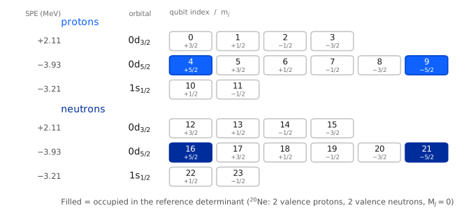
Every qubit is one -scheme single-particle state , and means occupied. The register uses a fixed order: protons first, then neutrons; within a species, orbitals in file order; within an orbital, descending. The two halves of a bitstring are therefore the proton configuration and the neutron configuration. This is the bipartition expected by the pooled SQD post-processing tools.
The workflow
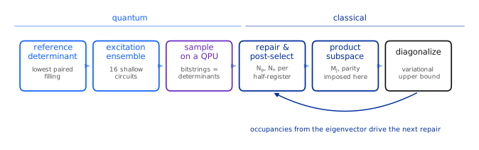
Two stages in the diagram handle the nuclear symmetries.
Repair and post-selection handle samples affected by hardware noise. The two half-register nucleon numbers
are Hamming weights, so qiskit-addon-sqd handles them directly: recover_configurations repairs a
broken bitstring by flipping the bits least consistent with the current estimate of the average
orbital occupancies, rather than throwing the shot away.
The product subspace introduces . Because couples the two halves, it is not a property of either one, so it must not be used to filter whole shots: a bitstring whose proton half and neutron half are each valid still contributes two good half-configurations even when its total is wrong. The subspace is therefore spanned by every product of a sampled proton configuration with a sampled neutron configuration, keeping the products that land in the target and parity sector. This is the pooled SQD subspace construction, and it means a few thousand bitstrings can span a subspace far larger than the sample count.
Two governing equations
The shell-model Hamiltonian is a one-body term plus a two-body interaction,
where label -scheme states and for a proton, for a neutron. Empirical interactions such as USDA [2] and GXPF1 [3] are tabulated not in the -scheme but in the -coupled basis, as matrix elements between normalized antisymmetrized two-body states of orbitals . Recovering the -scheme element is a Clebsch-Gordan recoupling,
with the factors undoing the normalization convention of the tabulated states. Everything else in this tutorial is built on these two equations.
The three runs
| Nucleus | Shell | Qubits | Symmetry-allowed basis | Exactly checkable? | |
|---|---|---|---|---|---|
| Small-scale | (2p + 2n) | 24 | 640 | Yes | |
| Large-scale | (2p + 2n) | 40 | 4,000 | Yes | |
| Large-scale | (4p + 4n) | 40 | 1,963,461 | No |
The small-scale run is the walkthrough. Both large-scale runs use a 40-qubit register: the first is still small enough to diagonalize exactly on a laptop, so you can compare the hardware result with an exact reference. The second exceeds the exact-diagonalization capacity of this tutorial.
Every run here executes on a QPU. That is a choice made for this tutorial rather than a requirement of the method: all three runs share a backend and a gate budget so you can compare their performance at different problem sizes.
Requirements
Install the following packages before starting:
- Qiskit SDK v2.0 or later (
pip install qiskit) qiskit-ibm-runtimev0.40 or later (pip install qiskit-ibm-runtime)- SQD addon v0.12 or later (
pip install qiskit-addon-sqd) - NumPy, SciPy, and Matplotlib (
pip install numpy scipy matplotlib)
You also need an IBM Quantum® account with credentials saved locally, and access to a QPU with at least 40 qubits.
No simulator package is needed, and no data files have to be downloaded. The two interaction files this tutorial uses are embedded in the following setup cell and written to a temporary directory when you run it.
Setup
This section imports the tools and defines the shell-model helpers the workflow needs, in the order the workflow uses them. The physics behind each one is derived in the Appendix; the comments describe each function’s role in the workflow.
Two interaction files are unpacked first. Both are published parameter sets, embedded here so the
notebook is self-contained: usda.snt is the USDA -shell Hamiltonian [2] and
gxpf1.snt is the GXPF1 -shell Hamiltonian [3].
# Added by doQumentation — required packages for this notebook
!pip install -q matplotlib numpy qiskit qiskit-addon-sqd qiskit-ibm-runtime scipy
from __future__ import annotations

import base64
import gzip
import itertools
import tempfile
from dataclasses import dataclass
from functools import lru_cache
from math import factorial, sqrt
from pathlib import Path

import matplotlib.pyplot as plt
import numpy as np

from qiskit import QuantumCircuit
from qiskit.circuit.library import PauliEvolutionGate
from qiskit.quantum_info import Operator, SparsePauliOp
from qiskit.transpiler.preset_passmanagers import generate_preset_pass_manager
from qiskit_addon_sqd.configuration_recovery import recover_configurations
from qiskit_addon_sqd.counts import bit_array_to_arrays
from qiskit_addon_sqd.subsampling import postselect_by_hamming_right_and_left
from qiskit_ibm_runtime import QiskitRuntimeService, SamplerV2

from scipy.linalg import eigh

_USDA_SNT_GZ = (
    "H4sIAI5wqWoC/4WY224bRwyG7/UU9F0CONsZco5AUyBuC/QmQNG06KWhWGql1LYMy+kJefiOTrucGXJrQAgsf5nl8ecOr+CX"
    "D9+9g/0K9pv1/T389rx7gPLrsH+Cz/vVctg+vgAsrgB+HeDdAD9t7zYv6+dr+DDA+z8223/X17B8XMFN+ev9+m+4ed799XjA"
    "f9z8sy/4+s8BvoWYrsEERwbhFRqTXi+uCvOwW63vYf+0vFvDAgDo/AFIh8/hK7DH30354Omvb8o3V8c/vIUnMKtboK/wiGKF"
    "+gnFEfVn9PQUe8bthNIRtftbsGfUtQbAGXUFfawM8K0BF9SP6MWA0BpwQcMRvRhwBSX86+fl3ct2d4jq4+eHa3hYv2x2q7fX"
    "AJuPy+fb3cP69+Uh4luAT8djv95++eGV/fj6y6dvFudnmcX4lGOoBmttNOVncTL2FLs3NGT0l++ndJTv0cR8/t6NUanP8WMI"
    "6nPC6C8/5wp+vnn//QLOP9ank3k2wRszkDn/Zwv15xiv41l2SDmjhuEFM4PJ0QkYcgzM4A1Jp1GDkcvtaWMAR9tosAa9huHk"
    "AtoUBYwaF8hGarAxOywgxnoeN+Se2smF4H3QMPZQ653XMJpOi6GyrcLcZJtzLgoYcdsOyXKibV1Aom0fikJO0VLUMDeW3kAl"
    "qQLWpd66qGE02eZ9lXqSPD3UWyl5DeOeGnINJnmaUggCVrtgh2DJNm3fVy8WF3LSMFa9hYga5iYX0IQsYK2nmTpJkoq81Acy"
    "jLTTnPEaxqo3JGcbvZMeGnJVbw6mf2cUqcIsO80nFdOFq8JoSlY+Zb7FfNNZlnw2PqOE8SL3PtlSJhJGXGqsDRjbh4bmocWy"
    "oiIxSxjv09JYgaxlGLZxA9EFFOImuIBt3EB04TK3Z5S8wizrrFCJQ4Xpgl9hzDYbu0LCNm6HzkJHweUkYazITalyF7NjGAnh"
    "FZJFQniFZFHnqWgbdZ6qtoX50VZhvEJ81TJe7AUcQozH8yQMJ8ymUS07jLin6LXT3FRIhmwSTmtbJpEjr2AsvM7E1ra+ZaiM"
    "NoxewZinBlPQTmPJyikn7TQ2630SbWuz4CLlwzuGhCHPqbUmRZQwpkiBDn1vsoQ55oKjbEvNNVgbXls0WvA0NKnPpku91Fkx"
    "pahhXPDJtxVCQkBcMtJD27I8VJGAhWYYlVuZzc5e+jSIZWnLa57nOQ1iWZY+jSE3GP5/QIKi5E1Agqi9BbMZiUjEWNwChqKq"
    "KTZY11ku5ca2Pqc4YKk1o2DstBjJC1htW2nAgEZ4aDdPvQmmmLeY4tWFt9Y3VAdlpW+oDcpa3zpM1jdUB2XV9agOyqrrcWZQ"
    "sq7vMMffBseux5l5yjoLZ+Yp6yzU5mmt5DgzT5mSozZPoVIknJmnTJFQHZRV12OrlvpFQFbycoGKOWiYfl9QlXySGtSUvL9W"
    "VJi/YG4grC4CmuCX6CZrKUsY64UyJolCQoZJqWeKhDOCzxQJNcGXbZMEX7EtzF+gvCI1npxjmKaW5Q06ewVjOY0u2+Y0kt5D"
    "JhlETS2P+5CqyIMYkCI1NK50SO3TarSR2qfVaKOZPmXjg2beVJmS01zqp/CSmvoqvNSOD/kaS+qUoSGaTM2yz83fdjtMvsZy"
    "xOv7N44Fff/GT5q5tXWYfB3jWND3b9yumUvK5SQnvK6w/VuHyfu3DpP3bx0m7984FvT9W4fJ+zceWq/v3zpM3r9xLOj7tw6T"
    "928X053QgGz/1mHy/u3yZ8lTtn/jWND3b74NiDx2vRbeep56Lbz1oPRaeOv9G0dmxofXPK33bx0m798C1B9RuP4DPJ0WcLAa"
    "AAA="
)

_GXPF1_SNT_GZ = (
    "H4sIAI5wqWoC/4WcQY8dtw3H7/kU41sCeF8lUqKkQw9NgbaXoEHQQ26BkdiIEWdt2E6L9tNXb9+ORIn8PwdZILB/S3I4IsW/"
    "ZiYvjr//+P3f4nG8ef/x+PDm4dOvr9+9++rF8d3l+Mf7x99fvTz+dTn++fnTH7/1//z28pfL8e3H9/95fHm8evzl+lffvf3f"
    "H59e/fb26L9zHN//+t9Pl+OH1/++HH89JL88gkQO8esfvjm+phDomyvW//39/S+v3x2fPrz6+fVX/dfS889B4fpz/aN43P7p"
    "f3Bw/ynH8fD0Zy+uf/fn48MR3vxU/kRXlp7Z+PzDiqUnNn74iW8sb3azYvm0m29s2uxGxabTbryx2cZ7nGzu7KOKV2y8g5Un"
    "dsZbbLyDLafd53irjXew9bR7jffF8fbx8+uPr37+/Pb941dPv3P93ZH4W/If6kUohXCm+Jbmh3yR0jicybwl9CFeuFILy908"
    "HtIlcrlZyCNJ2q6MdGi7ZVy4tlvHJS52Y71FnHp8D+HCIYTlQuYFhdsv0yVxzZB6vsxwaZwJUumkIjWB1POdDhcqlR2KVo85"
    "SoDU8NgdNodiZevqMUqB1LCVWsO2ZMQlyYs+bXEFk4m5bMJJlVgSpGjaouhQvFKxUIbUjIvI85hWW4FNvubyDnMxMkFKRc8V"
    "Uml65OhQW1x9fe3XOAtsZPXJ36TIX18SaoQUnysnZsHUXPfcKqTyaSu36FHbWg0tN0jxWIXEAVLzbqcqkMpj3T8lwlBp9RhD"
    "qpAaHpnzni9nRXPh6lDbysmJBVLzDtU71KztnDxqW1+JhDaKnTtUa4DUzH00Hp0VXQMHSM3c16irlpf7GEcN1dogpfpEDpAa"
    "WRUOBKl0UqkIQ2qs+5IYU6OvthbFodIaF6/9i51VeF0TLZSN2lfh9T729utQOqtXKi/dl/21mihhW+M+BpIKqblypDWHSntc"
    "mSA1O3nMe+6dHp0DEaRmXCU0h9p7dOYCqVm1MehOnvy7nWphSKnuu+Q++X2Ca4uQGrYkxp3yMkFLL0ygavPovmR64dhFY5QM"
    "KVK1XRxqX4UydlHCXU44hY1ydndKuUBK11BzqH1NNOKNMvt27PMXVUWBemSqCVIjrr4nYFtzTSQJkJp3O7se09p9YygCKVL7"
    "UN4opx5DNnE5q5AlerZ2jyExpEYmggTtMYFrzC1Bak58jetGeSvHenSip9ROik0m5lqdsxzjrCYhTM1uImOHYZzVPvnWjXIm"
    "0RoaKyqhjjlqiEE3uWoYHqopbT/KY0pDD+Xtx9d8lvI0n6U8zWcpT/NpQqDms5Sn+TRVoOazlKf5LOVpPk1VqPl05AI1n6U8"
    "zaepAjWfpTzNp6kKNZ/OQoGaz1Ke5rOUp/k0VaHm03mvUPOd1+esL6X5LOVpPkt5ms9SnubTVIGaz1Ke5rOUp/ks5Wk+TVWo"
    "+SzlaT69mgVqPk0VqPks5Wk+S3maT1MVaj5dPwVqPkt5mk9TFWo+S3ma77x/8z56ms9SnuazlKf5LOVpPkt5ms9SnubTVIWa"
    "z1Ke5jupfRWumk9TBWo+S3maz1Ke5rOUp/k0VaHms5Sn+XTnLVDzWcrTfJqqUPNZytN85/1z7rbSfJbyNN/5t06fUJrPUp7m"
    "OykvE7T0wgqqdmo+Mb3Q03yCO6bSfII7ptJ8gruc0nxi+pen+eROL5yaT3CXU5pPx1Sh5hNcj0rzCajHVfMJqMdV88mdesyu"
    "xwo1n+B6VJpPcD0qzSe4HpXmE1yPSvMJrkelwERVR4Waz1Ke5hNTQ3THoxO90nzFZMLTfAVnVWm+grOqNF/BWVWaTxMVar6C"
    "r1FpvgK6yar56vbja76onormu8/5ViqOrNblZH6l0NPAlRq9sKaIbaFnhis15tUuH/E1oieLK1XOTIgsz3ROap9XpQ/SJWqK"
    "bCYcKm6K4tp9iUqqzbd1j4qO+g2tpTV6sll1qLipk6fnw32/isDWPSruPborwz7x9eakKbbry6Gi7RN9nrhuHr4tPXXsVLT9"
    "vvTdKlUQ18i9Q0Wn+2ZOlYpva0yiDhXthNz69p4S+7ZG7h0q2jma+/BIIfm2RnU4VLQ9R6hG4iWryVurhorOlNbzEJr4tubk"
    "bim6e25iqbFbJY4MKfREfaXGNXKK2aF2BSapD6Oy5162yd1S5Og0iq3k5tua1WEpsus+ZO4ZS76tqU4sRc7+mAtJyL6teR8t"
    "RVbDUO9yXM2a2O6jQ5GjdCi3HKpva04dluK7J1uWGtFLjhFS6J2HlZpKhzOm0JsRK5XnmjD7Izv5av0eBd7zVb5IsVU6ffTN"
    "oQXf1peoeveNjZWaNURFZ0L8fTsX1s9hwO4eeHkOA3Z3Zct6ZOccgPAM0O91hR4ZPEcWMAPkdBWQvsdZj72xZuTRs2U95qFY"
    "a8FZHVQpy/Mhd55YbGmPew2VGB2PRvOVsNlib0orYbO1U8fi0cbF6uQhw7jUycMybYs/dSiKwGxyLB5tXEmdM5WM4lKnGLFm"
    "FFeaPTruK8ehlEcbV55n2yIwrnlOXorAuPKsxyIwrjz7l3greptzSgve+tqo2lLbcu9MQ4oiPDMpjzaueR8rUUZxqaql/T46"
    "k5WiCM9fyuNpy5uZpM9WkvfaxpS1Ndd96JKV2LflUdrW1idaKOT0HNMnTCdnT/OZvcOZv5RHG5fqAJFhXLO2WykwrtlzJkV4"
    "llMebVxp7kOUMopr7h1dSmcUl9LuxesT2z6kPOq4ttkkk7sj1/1JWWWnHvfdfVKE50LlUV+jObPqs2hO+zViytpSJ+CFSyu+"
    "LY+yttRM3gf3HH1bHmVtzR5NXZQXcI0epW1tdyh2d86a2O52F9vR6V8FUgTm1dWjjWuepZUgMK45k2cKMC6PIjD7rh6j+gpi"
    "0Y904b675/n2h3u6QteTedkoc7qy2LIeaUxpkXNAHgeV53khozOYxZb1qDpTrvAa+TxBClECvEbPlvWY5o4cA7zGNDSfFIbX"
    "6NmyHmd1SEnwGgfVJ6YKr9GzZT3KebdDZIYe5bzGQLFAj54t7XHXfDkmJ6v789r17e7iTEMrxXhmUh5tXHNmainCuObMVBOO"
    "y6MYzEyrx9MW2VMf4cC9NWlbzpmVoqytucPkIO12SsZ4/lKUtTX7V6LGsfi2phadlLa1nX89naUHc437uYnQni/nlEzWN/S8"
    "s7TVo41LvUsW9+pwqFBl79HsPYkVr/sK9GjjYnVWSzBfqjoowXx5FN+ZC6dHG5d6WybjfM15ouYE8+VRDObC1aOOa3v+WEJq"
    "Tlzb2VCRELOtbYEU47NH5dHGpd5nagzj0s+HAozLoxjMq6tHnfutHmNjblz23G/1qChra3rMOT6f3jGefRVlbamZKfR1COKa"
    "PWdS1tZcXy3mnMm3pd4IGpS1Nd9Uai0Wir6t+fxxUtrWPvu27M1MG8XJ1KMz+yqK8Vmt8mjjmn1CKmcUF88zhVIzimtOtZNi"
    "fO6rPGpbW9XGLrg50G5rfwNhUueu7swmEtI55yQ0m/RpqI3JPd15ujVtWY9TSbcxpSU8dSShAj16tk4b3r6dmUlI2/L27Ulp"
    "W7vKLFK3uByK4nI2VP19SFEJ7EOrRxvXyESr413YhPchLsssV/0dRlEJ70PKo7a1n/vWa1rLbsu8mTooa0up8tpyEd+Wep42"
    "KG1rf6su5ebkvpqztLzl3qltRSVc28ojmTM+9F2TwNm3Qgp9/eSeKnaNXFtwqH3nk1KaJE05M6ZDOdNjv9NJIvm2Zr+3lFeP"
    "EvqGnH1bM/eWMtNQvFCRHnzUlJlzXMqZYFKqHHLxbdFUFIbiu+8XWmo+50vL6R06l1u/PBO/asN8B5zAmdXTDtP7r8h+jeWL"
    "lFOPocYumti39SWq3v0iTvxdtDw9hhmUq9N6PbaqvzJyqyNeMi0nIm51LLbojgIrOUKP+l2yBj16tghrqxib1gqg0pLknfIq"
    "bdoirJqkMMNrnDNATPgaPVuE9VBv0J7HbU107V42W44eUhSjPrF4JKyHUokZxqXeTV+exAI9pCjGp/zKIwE9dO2+XSTX1vbc"
    "b6pJUYT1UOCWWw2+rdmZJkVYD1Ef0Uoi39acySdFWA9RztLVjm9LPQ0cFAENc3unJjrVsWuY0mK297EYxbrbcs7vlUfCGib3"
    "bQ/GNWffMijCGkZRDHr0w+KRsIbpnem6dnZbe9VOitTsW7e3I+e7Pgnv7tfHQxvl7O7KlvU4zu95fouUUNV21RSGFk2oHhdb"
    "ZGbf+b4cXf8nRlnb8maASVlbc+UkSnSb0hKox4eFIjNHz7c/aHydkvC6T9Lydo3Je+u8ZSdf+xsu06O2ta2vPr70W1l2W9v6"
    "UhSbPoG+kwYnSDVnTKGvqYvfv3JuDVLom2vvpOZpvh9fizHuX71jVp79vqDcG8rrJolLnecTxe8TgMLfBTDoJteOGUVntYJr"
    "5PHOVsKnUaEuJw8oE9MWA5V5e2tA9wmQrw5xQB6RrernS33VkEB1PCmKW5f7P6zudeW7TwAA"
)

DATA = Path(tempfile.mkdtemp(prefix="nuclear_sqd_"))
for name, blob in (("usda.snt", _USDA_SNT_GZ), ("gxpf1.snt", _GXPF1_SNT_GZ)):
    (DATA / name).write_bytes(gzip.decompress(base64.b64decode(blob)))

    if not (DATA / name).is_file():
        raise RuntimeError(f"{name} did not unpack to {DATA}")
The model space and the qubit register
An .snt file holds the model space, the single-particle energies, and the -coupled two-body
matrix elements. For the mass-dependent interactions used here, the third and fourth fields of the two-body
header specify the reference mass
at which the interaction was fitted and the exponent of its mass dependence. Both
files carry the exponent , with for USDA and for GXPF1, so the
tabulated matrix elements must be rescaled by for the nucleus being
computed [2], [3]. Single-particle energies are not rescaled. Skipping
this step changes the correlation energy by a few percent.
The energies that follow are valence energies, measured from the inert core; they are not experimental separation energies.
@dataclass(frozen=True)
class Orbital:
    idx: int
    n: int
    ell: int
    j2: int
    tz: int  # j2 = 2j; tz = -1 proton, +1 neutron

@dataclass(frozen=True)
class SPState:
    """One m-scheme single-particle state, i.e. one qubit."""

    orb: int
    j2: int
    mj2: int
    tz: int
    ell: int
    spe: float  # mj2 = 2 * m_j

@dataclass
class ModelSpace:
    orbitals: list
    spes: dict
    tbmes: dict
    core_z: int
    core_n: int
    mass_number: int
    a_ref: int
    mass_exponent: float
    mass_factor: float

def read_snt(path, n_protons, n_neutrons):
    """Parse a .snt interaction file, applying its mass dependence for this nucleus.

    The two-body header line is ``n_tbme  method  A_ref  exponent``.  When ``method`` is 1 the
    tabulated matrix elements are rescaled by ``(A / A_ref) ** exponent``, where A is the mass
    number of the whole nucleus -- the core plus the valence nucleons.  A is derived from the
    file's own core numbers rather than passed in, so it cannot silently disagree with the
    valence counts the rest of the workflow uses.  Single-particle energies are not rescaled.
    """
    rows = [
        ln.split("!")[0].split() for ln in Path(path).read_text().splitlines()
    ]
    rows = iter([r for r in rows if r])

    n_p_orb, n_n_orb, core_z, core_n = (int(x) for x in next(rows)[:4])
    orbitals = [
        Orbital(*(int(x) for x in next(rows)[:5]))
        for _ in range(n_p_orb + n_n_orb)
    ]

    spes = {}
    for _ in range(int(next(rows)[0])):  # "i  i  <i|H(1b)|i>"
        field = next(rows)
        spes[int(field[0])] = float(field[2])

    n_tbme, method, a_ref, exponent = next(rows)[:4]
    n_tbme, method, a_ref, exponent = (
        int(n_tbme),
        int(method),
        int(a_ref),
        float(exponent),
    )
    mass_number = core_z + core_n + n_protons + n_neutrons
    factor = (mass_number / a_ref) ** exponent if method == 1 else 1.0

    tbmes = {}
    for _ in range(n_tbme):  # "a  b  c  d  J  value"
        field = next(rows)
        tbmes[tuple(int(x) for x in field[:5])] = float(field[5]) * factor

    return ModelSpace(
        orbitals,
        spes,
        tbmes,
        core_z,
        core_n,
        mass_number,
        a_ref,
        exponent,
        factor,
    )

def m_scheme_states(ms):
    """The qubit register: protons then neutrons, orbitals in file order, m_j descending."""
    return [
        SPState(o.idx, o.j2, m2, o.tz, o.ell, ms.spes[o.idx])
        for tz in (-1, +1)
        for o in ms.orbitals
        if o.tz == tz
        for m2 in range(o.j2, -o.j2 - 1, -2)
    ]
Clebsch-Gordan recoupling
Equation (2) requires Clebsch-Gordan coefficients for half-integer angular momenta. Every argument is
passed as twice its physical value, so enters as 5 and the arithmetic stays exact.
Interaction.v_ms handles lookups of the interaction matrix elements. An .snt file stores each
matrix element once, so a lookup might need the antisymmetrized pair-exchange phase on either
side, and the bra and ket might be stored in either order.
@lru_cache(maxsize=None)
def clebsch_gordan(j1_2, j2_2, J_2, m1_2, m2_2, M_2):
    """<j1 m1 j2 m2 | J M>.  Every argument is twice its physical value."""
    if m1_2 + m2_2 != M_2 or not abs(j1_2 - j2_2) <= J_2 <= j1_2 + j2_2:
        return 0.0
    if abs(m1_2) > j1_2 or abs(m2_2) > j2_2 or abs(M_2) > J_2:
        return 0.0
    if (j1_2 + j2_2 - J_2) % 2 or (j1_2 - m1_2) % 2 or (j2_2 - m2_2) % 2:
        return 0.0

    f, half = factorial, lambda x: x // 2
    prefactor = sqrt(
        (J_2 + 1)
        * f(half(j1_2 + j2_2 - J_2))
        * f(half(j1_2 - j2_2 + J_2))
        * f(half(-j1_2 + j2_2 + J_2))
        / f(half(j1_2 + j2_2 + J_2) + 1)
        * f(half(J_2 + M_2))
        * f(half(J_2 - M_2))
        * f(half(j1_2 - m1_2))
        * f(half(j1_2 + m1_2))
        * f(half(j2_2 - m2_2))
        * f(half(j2_2 + m2_2))
    )
    total = 0.0
    for k in range(half(j1_2 + j2_2 - J_2) + 1):
        d = [
            half(j1_2 + j2_2 - J_2) - k,
            half(j1_2 - m1_2) - k,
            half(j2_2 + m2_2) - k,
            half(J_2 - j2_2 + m1_2) + k,
            half(J_2 - j1_2 - m2_2) + k,
        ]
        if all(x >= 0 for x in d):
            total += (-1) ** k / (
                f(k) * f(d[0]) * f(d[1]) * f(d[2]) * f(d[3]) * f(d[4])
            )
    return prefactor * total

class Interaction:
    """Antisymmetrized m-scheme two-body matrix elements <pq||rs>, per Eq. (2)."""

    def __init__(self, model_space, sp):
        self.ms, self.sp, self._cache = model_space, sp, {}

    def _tbme(self, oa, ob, oc, od, J, j_ab_2, j_cd_2):
        """<oa ob; J|V|oc od; J>, allowing for how the file happens to order each pair."""
        table = self.ms.tbmes
        # |ba; J> = -(-1)^(j_a + j_b - J) |ab; J> for a normalized antisymmetrized pair;
        # dropping the leading minus makes v_ms symmetric instead of antisymmetric, and
        # the Hamiltonian then fails the rotational-invariance check in Step 1.
        phase_ab = -1.0 if (j_ab_2 // 2 - J) % 2 == 0 else 1.0
        phase_cd = -1.0 if (j_cd_2 // 2 - J) % 2 == 0 else 1.0
        for keys, phase in (
            (((oa, ob, oc, od), (oc, od, oa, ob)), 1.0),
            (((ob, oa, oc, od), (oc, od, ob, oa)), phase_ab),
            (((oa, ob, od, oc), (od, oc, oa, ob)), phase_cd),
            (((ob, oa, od, oc), (od, oc, ob, oa)), phase_ab * phase_cd),
        ):
            for key in keys:
                value = table.get(key + (J,))
                if value is not None:
                    return value * phase
        return 0.0

    def v_ms(self, p, q, r, s):
        """<pq||rs>, zero unless M_J and charge are conserved."""
        cached = self._cache.get((p, q, r, s))
        if cached is not None:
            return cached

        P, Q, R, S = (self.sp[i] for i in (p, q, r, s))
        value = 0.0
        if P.mj2 + Q.mj2 == R.mj2 + S.mj2 and P.tz + Q.tz == R.tz + S.tz:
            M = P.mj2 + Q.mj2
            # sqrt(1 + delta): undo the normalization of the tabulated pair states
            c12 = sqrt(2.0) if (P.tz == Q.tz and P.orb == Q.orb) else 1.0
            c34 = sqrt(2.0) if (R.tz == S.tz and R.orb == S.orb) else 1.0
            for J2 in range(
                max(abs(P.j2 - Q.j2), abs(R.j2 - S.j2)),
                min(P.j2 + Q.j2, R.j2 + S.j2) + 1,
                2,
            ):
                cg_bra = clebsch_gordan(P.j2, Q.j2, J2, P.mj2, Q.mj2, M)
                cg_ket = clebsch_gordan(R.j2, S.j2, J2, R.mj2, S.mj2, M)
                if abs(cg_bra) < 1e-12 or abs(cg_ket) < 1e-12:
                    continue
                value += (
                    c12
                    * c34
                    * cg_bra
                    * cg_ket
                    * self._tbme(
                        P.orb,
                        Q.orb,
                        R.orb,
                        S.orb,
                        J2 // 2,
                        P.j2 + Q.j2,
                        R.j2 + S.j2,
                    )
                )

        self._cache[(p, q, r, s)] = value
        return value
Matrix elements and the symmetry test
A determinant is a sorted tuple of occupied qubit indices. Two determinants differing in more than two occupied states have a vanishing matrix element; otherwise, the Slater-Condon rules give a short sum over the interaction, multiplied by a fermionic sign counting how many occupied states lie between the operators in the fixed register ordering.
symmetry_allowed is the integer test that all four exact quantum numbers reduce to. It is used both
to filter samples and to enumerate the exact basis for the runs small enough to check.
def matrix_element(inter, det_a, det_b):
    """<A|H|B> for two determinants, each a sorted tuple of occupied qubit indices."""
    set_a, set_b = set(det_a), set(det_b)
    out_a, out_b = sorted(set_a - set_b), sorted(set_b - set_a)
    if len(out_a) != len(out_b) or len(out_a) > 2:
        return 0.0

    if not out_a:  # diagonal: one-body plus two-body
        return sum(inter.sp[i].spe for i in det_a) + sum(
            inter.v_ms(i, j, i, j)
            for i, j in itertools.combinations(det_a, 2)
        )

    if len(out_a) == 1:  # one state moves, p -> q
        p, q = out_a[0], out_b[0]
        crossings = sum(1 for k in set_a if min(p, q) < k < max(p, q))
        return (-1.0) ** crossings * sum(
            inter.v_ms(p, j, q, j) for j in det_a if j not in (p, q)
        )

    (p, r), (q, s) = out_a, out_b  # two states move
    crossings = sum(1 for k in set_a if p < k < r) + sum(
        1 for k in set_b if q < k < s
    )
    return (-1.0) ** crossings * inter.v_ms(p, r, q, s)

def subspace_hamiltonian(inter, dets):
    """Dense real-symmetric H projected onto the span of `dets`."""
    H = np.zeros((len(dets), len(dets)))
    for a, det_a in enumerate(dets):
        H[a, a] = matrix_element(inter, det_a, det_a)
        for b in range(a + 1, len(dets)):
            H[a, b] = H[b, a] = matrix_element(inter, det_a, dets[b])
    return H

def ground_state(inter, dets):
    """Lowest eigenvalue and eigenvector of H over `dets`."""
    values, vectors = np.linalg.eigh(subspace_hamiltonian(inter, dets))
    return values[0], vectors[:, 0]

def symmetry_allowed(
    sp, det, n_protons, n_neutrons, mj2_target=0, parity_target=0
):
    """The four exact shell-model quantum numbers, as integer tests on one determinant."""
    n_p = sum(1 for i in det if sp[i].tz == -1)
    return (
        n_p == n_protons
        and len(det) - n_p == n_neutrons
        and sum(sp[i].mj2 for i in det) == mj2_target
        and sum(sp[i].ell for i in det) % 2 == parity_target
    )

def full_basis(sp, n_protons, n_neutrons, **targets):
    """Every symmetry-allowed determinant.  Only tractable for small model spaces."""
    protons = [i for i, s in enumerate(sp) if s.tz == -1]
    neutrons = [i for i, s in enumerate(sp) if s.tz == +1]
    return [
        p + n
        for p in itertools.combinations(protons, n_protons)
        for n in itertools.combinations(neutrons, n_neutrons)
        if symmetry_allowed(sp, p + n, n_protons, n_neutrons, **targets)
    ]

def count_basis(sp, n_protons, n_neutrons, mj2_target=0, parity_target=0):
    """How many determinants `full_basis` would return, without enumerating them.

    A dynamic program over (occupied count, sum of 2*m_j, parity) per species.  This stays
    cheap when the basis itself is far too large to build, which is how the largest run below
    can report the size of the space it is sampling from.
    """

    def species(states, k):
        table = {(0, 0, 0): 1}
        for s in states:
            for key, value in list(table.items()):
                count, m_sum, parity = key
                if count < k:
                    nxt = (count + 1, m_sum + s.mj2, (parity + s.ell) % 2)
                    table[nxt] = table.get(nxt, 0) + value
        totals = {}
        for (count, m_sum, parity), value in table.items():
            if count == k:
                totals[(m_sum, parity)] = (
                    totals.get((m_sum, parity), 0) + value
                )
        return totals

    left = species([s for s in sp if s.tz == -1], n_protons)
    right = species([s for s in sp if s.tz == +1], n_neutrons)
    return sum(
        a * b
        for (mp, pp), a in left.items()
        for (mn, pn), b in right.items()
        if mp + mn == mj2_target and (pp + pn) % 2 == parity_target
    )
The reference determinant
The ansatz is built on top of a single determinant, so that determinant should be the best one available. Filling the lowest single-particle energies ignores the two-body interaction. In these model spaces, that choice gives an energy 1–2 MeV above the lowest-energy determinant.
Restricting to fillings made of time-reversed pairs forces exactly and leaves only candidates per species (a few thousand at most), so the best one can be found by searching them all on the full diagonal . Ties go to the most strongly aligned pairs, where the pairing force is strongest. In every case in this tutorial that can be checked against a full enumeration, the search returns the global lowest-diagonal determinant, which is also the largest single component of the exact ground state.
def reference_determinant(sp, inter, n_protons, n_neutrons):
    """Lowest-diagonal determinant built from time-reversed (+m_j, -m_j) orbital pairs."""
    if n_protons % 2 or n_neutrons % 2:
        raise ValueError(
            "an odd valence count has no time-reversed paired reference at M_J = 0"
        )

    def species_pairs(tz):
        return [
            (
                q,
                next(
                    p
                    for p, t in enumerate(sp)
                    if t.tz == tz and t.orb == s.orb and t.mj2 == -s.mj2
                ),
            )
            for q, s in enumerate(sp)
            if s.tz == tz and s.mj2 > 0
        ]

    best = None
    for chosen_p in itertools.combinations(species_pairs(-1), n_protons // 2):
        protons = tuple(q for pair in chosen_p for q in pair)
        for chosen_n in itertools.combinations(
            species_pairs(+1), n_neutrons // 2
        ):
            det = tuple(
                sorted(protons + tuple(q for pair in chosen_n for q in pair))
            )
            # break ties toward the most aligned pairs, where J = 0 pairing is strongest
            score = (
                matrix_element(inter, det, det),
                -sum(abs(sp[q].mj2) for q in det),
            )
            if best is None or score < best[0]:
                best = (score, det)
    return best[1]
The excitation pool and its perturbative ranking
Correlation is carried by two-particle–two-hole () excitations from the reference. Two selection rules reduce the pool before any circuit is built: an excitation must conserve , and the hole pair and particle pair must be able to couple to a common total , which is a triangle inequality.
The remaining excitations are ranked by the Epstein-Nesbet second-order score of selected configuration interaction [4],
which estimates how much correlation energy each excitation carries. The same two numbers fix the circuit angle: with , the first-order amplitude is . The Appendix explains why the first-order amplitude is the choice used in this tutorial rather than the exact two-level angle.
def excitation_pool(sp, occ):
    """2p2h quadruples (h1, h2, v1, v2): same-species pairs, then proton-neutron pairs."""
    holes = {tz: [i for i in occ if sp[i].tz == tz] for tz in (-1, +1)}
    virtuals = {
        tz: [i for i, s in enumerate(sp) if s.tz == tz and i not in occ]
        for tz in (-1, +1)
    }
    pool = [
        (h1, h2, v1, v2)
        for tz in (-1, +1)
        for h1, h2 in itertools.combinations(holes[tz], 2)
        for v1, v2 in itertools.combinations(virtuals[tz], 2)
    ]
    pool += [
        (h1, h2, v1, v2)
        for h1 in holes[-1]
        for h2 in holes[+1]
        for v1 in virtuals[-1]
        for v2 in virtuals[+1]
    ]
    return pool

def conserves_symmetry(sp, op):
    """Keeps M_J, and the hole and particle pairs share a reachable total J."""
    h1, h2, v1, v2 = op
    if sp[v1].mj2 + sp[v2].mj2 != sp[h1].mj2 + sp[h2].mj2:
        return False
    return max(abs(sp[v1].j2 - sp[v2].j2), abs(sp[h1].j2 - sp[h2].j2)) <= min(
        sp[v1].j2 + sp[v2].j2, sp[h1].j2 + sp[h2].j2
    )

def en_denominator(inter, occ, holes, virtuals, floor=0.1):
    """Epstein-Nesbet gap: bare gap, spectator rearrangement, and the pair's own term."""
    gap = sum(inter.sp[h].spe for h in holes) - sum(
        inter.sp[v].spe for v in virtuals
    )
    for k in occ:
        if k in holes:
            continue
        gap += sum(inter.v_ms(h, k, h, k) for h in holes)
        gap -= sum(inter.v_ms(v, k, v, k) for v in virtuals)
    gap += inter.v_ms(holes[0], holes[1], holes[0], holes[1])
    gap -= inter.v_ms(virtuals[0], virtuals[1], virtuals[0], virtuals[1])
    return gap if abs(gap) >= floor else (floor if gap >= 0 else -floor)

def rank_pool(inter, occ, pool):
    """Sort by descending PT2 score; return (operator, coupling, first-order amplitude)."""
    ranked = []
    for op in pool:
        h1, h2, v1, v2 = op
        coupling = inter.v_ms(v1, v2, h1, h2)
        gap = en_denominator(inter, occ, (h1, h2), (v1, v2))
        ranked.append((coupling**2 / abs(gap), op, coupling, coupling / gap))
    ranked.sort(key=lambda row: (-row[0], row[1]))  # deterministic on ties
    return [
        (op, coupling, amplitude) for _, op, coupling, amplitude in ranked
    ]
Qubit-excitation blocks
Under the Jordan-Wigner mapping a particle-conserving excitation operator becomes a sum of eight Pauli strings, each carrying a string of operators between the outermost indices. The strings enforce fermionic antisymmetry, and they are expensive: a proton-neutron excitation spans the boundary between the two halves of the register and includes a parity string across that boundary.
Dropping the strings gives the qubit-excitation operator of Yordanov et al. [5]. The state prepared by this operator has different amplitudes, but it connects exactly the same pairs of determinants, so the set of determinants the circuit can reach is unchanged. Pooled SQD uses these determinants for the classical diagonalization. Step 2 compares the support of the two constructions and measures their hardware costs.
Building the Pauli form from , with the
string optional, keeps the two constructions a single flag apart. All eight terms of one generator
commute, so a single PauliEvolutionGate step is the exact exponential rather than a Trotter
approximation to it.
def _ladder(num_qubits, q, dagger, parity):
    """Pauli form of a_q or a_q^dagger.  `parity` toggles the Jordan-Wigner Z string."""
    prefix = (
        ["Z"] * q + ["I"] * (num_qubits - q) if parity else ["I"] * num_qubits
    )
    x_part, y_part = list(prefix), list(prefix)
    x_part[q], y_part[q] = "X", "Y"
    return SparsePauliOp(
        ["".join(reversed(x_part)), "".join(reversed(y_part))],
        coeffs=[0.5, 0.5 * (-1j if dagger else 1j)],
    )

def excitation_generator(num_qubits, op, parity=False):
    """Hermitian H with exp(-i theta H) = exp(theta (T - T^dagger)) for T = a+ a+ a a."""
    h1, h2, v1, v2 = op
    T = SparsePauliOp("I" * num_qubits)
    for q, dagger in ((v1, True), (v2, True), (h2, False), (h1, False)):
        T = (T @ _ladder(num_qubits, q, dagger, parity)).simplify()
    return (1j * (T - T.adjoint())).simplify()

def excitation_block(op, theta, parity=False):
    """(window, circuit) for one excitation.

    A qubit excitation touches only its four qubits.  A fermionic excitation also carries Z
    operators on every qubit between the outermost indices, so its window is the whole span --
    which is exactly where its extra cost comes from.
    """
    window = list(range(min(op), max(op) + 1)) if parity else sorted(op)
    local = tuple(window.index(i) for i in op)
    generator = excitation_generator(len(window), local, parity=parity)
    return window, PauliEvolutionGate(generator, time=theta).definition

def excitation_ansatz(
    num_qubits, occ, operators, amplitudes, measure=True, parity=False
):
    """X gates for the reference determinant, then one evolution block per excitation."""
    qc = QuantumCircuit(num_qubits)
    for q in occ:
        qc.x(q)
    for op, theta in zip(operators, amplitudes):
        if abs(theta) < 1e-12:
            continue
        window, block = excitation_block(op, theta, parity=parity)
        qc.compose(block, qubits=window, inplace=True)
    if measure:
        qc.measure_all()
    return qc
The depth budget and the circuit ensemble
A single deep circuit containing every ranked excitation can exceed the hardware’s coherence time. Spreading the pool over an ensemble of shallow circuits and pooling their shots into one determinant set turns Step 2 into a packing problem: each excitation has a measured cost, each circuit has a budget, and the question is how much of the ranked pool fits.
The budget is measured in two-qubit depth (layers of two-qubit gates on the critical path) rather than in a raw gate count, because depth sets the circuit's duration and therefore how much of the device's coherence it spends. The total count is reported alongside it, since that is the better proxy for accumulated gate error; the two answer different questions and neither substitutes for the other.
Both quantities are extracted by arity: an instruction acting on exactly two qubits, whatever the backend happens to call its entangling gate. Matching on gate names instead could return zero for an unfamiliar basis set, incorrectly placing the whole pool in one circuit without exceeding the computed budget.
Filling whichever circuit is currently emptiest, in rank order, keeps every circuit near the budget. Costs are measured on the real backend target, one excitation at a time, because a cost read off an abstract circuit is not the cost the transpiler produces.
DIRECTIVES = ("barrier", "delay")

def is_two_qubit(instruction):
    """True for an operation on exactly two qubits, excluding directives.

    Selecting by arity rather than by gate name keeps this correct on any backend, whatever its
    two-qubit basis gate happens to be called -- cz on today's Heron devices, ecr on Eagle, or
    something newer tomorrow.  A gate-name allow-list silently returns zero on anything it has
    not heard of, which would collapse the whole pool into one circuit and pass every budget
    check.  Barriers are excluded because a barrier spanning two qubits is not a gate.
    """
    return (
        len(instruction.qubits) == 2
        and instruction.operation.name not in DIRECTIVES
    )

def two_qubit_count(qc):
    """How many two-qubit gates the circuit contains: the accumulated-gate-error proxy."""
    return sum(1 for instruction in qc.data if is_two_qubit(instruction))

def two_qubit_depth(qc):
    """Layers of two-qubit gates on the critical path: the duration and decoherence proxy.

    This is what the budget is measured in.  Two gates on disjoint qubit pairs run in the same
    layer, so depth tracks how long the circuit takes -- and therefore how much coherence it
    spends -- while the count above tracks how much gate error it accumulates.  Both are
    reported; only depth is budgeted.
    """
    return qc.depth(filter_function=is_two_qubit)

def excitation_costs(num_qubits, ranked, pm, parity=False):
    """Transpiled two-qubit depth of each excitation on its own."""
    return [
        two_qubit_depth(
            pm.run(
                excitation_ansatz(
                    num_qubits, (), [op], [amp], measure=False, parity=parity
                )
            )
        )
        for op, _, amp in ranked
    ]

def pack_ensemble(
    num_qubits, occ, ranked, costs, budget, n_circuits, parity=False
):
    """Fill n_circuits in rank order, always adding to whichever is currently emptiest."""
    bins, loads = [[] for _ in range(n_circuits)], [0] * n_circuits
    for (op, _, amplitude), cost in zip(ranked, costs):
        emptiest = min(range(n_circuits), key=lambda b: loads[b])
        if loads[emptiest] + cost > budget:
            break  # every circuit is full
        bins[emptiest].append((op, amplitude))
        loads[emptiest] += cost
    circuits = [
        excitation_ansatz(
            num_qubits,
            occ,
            [o for o, _ in b],
            [a for _, a in b],
            parity=parity,
        )
        for b in bins
    ]
    return circuits, bins

def pack_to_budget(
    num_qubits, occ, ranked, costs, budget, n_circuits, pm, attempts=6
):
    """Pack, transpile, and shrink the target until the assembled circuits really fit.

    Costs are measured one excitation at a time, but excitations that share qubits neither add
    nor parallelize cleanly once the transpiler routes them together, so the assembled depth is
    not the sum of its measured parts.  This loop closes that gap against the real transpiler,
    and it runs entirely before any job is submitted -- a budget failure must never cost shots.
    """
    target = budget
    for attempt in range(attempts):
        circuits, bins = pack_ensemble(
            num_qubits, occ, ranked, costs, target, n_circuits, parity=False
        )
        isa = pm.run(circuits)
        worst = max(two_qubit_depth(c) for c in isa)
        if worst <= budget:
            return circuits, bins, isa
        target = max(min(costs), int(target * budget / worst * 0.95))
    raise RuntimeError(
        f"could not fit {n_circuits} circuits inside a two-qubit depth of {budget} in "
        f"{attempts} attempts; raise N_CIRCUITS or DEPTH_BUDGET and re-run this cell. "
        "No QPU time was spent."
    )
Post-processing: repair, recombine, diagonalize
Three helpers do the work of Step 4.
half_configurations splits each sampled row into a proton half and a neutron half, and keeps each
half that has the correct nucleon number. A row with a valid proton half contributes that half even if its
neutron half has the wrong nucleon number. Each half carries the total sampled weight of the rows it appeared in, which
is what ranks it if the subspace needs to be truncated.
grow_subspace recombines the halves into every product that lands in the target and parity
sector, adding to the subspace it is given rather than rebuilding it. That keeps successive
subspaces nested, which is what makes the energy sequence monotone non-increasing instead of merely
fluctuating around a bound.
recovery_loop is the self-consistent configuration recovery of the pooled SQD paper
[1]: repair the two half-register nucleon numbers against the current occupancy
estimate, recombine, diagonalize, and take the next occupancy estimate from the eigenvector.
Check the bit-ordering conventions carefully to avoid incorrect results. qiskit-addon-sqd writes column 0 of its
bitstring matrix as the highest qubit index, so reversing a row gives occupation indexed by qubit;
its "right" half is the low qubit indices, which is the proton block. Correspondingly,
recover_configurations takes num_elec_a as the proton number and average occupancies ordered
(protons, neutrons) by qubit index. The addon assumes bit pairs with bit ; in this
register, proton qubit and neutron qubit are the same state, so the
assumption is physically meaningful here rather than incidental.
def half_configurations(
    bitstring_matrix, probabilities, sp, n_protons, n_neutrons
):
    """Split each row into proton and neutron halves, keeping each half on its own weight.

    Column 0 of the addon's matrix is the highest qubit index, so reversing a row gives
    occupation indexed by qubit.
    """
    protons, neutrons = {}, {}
    for row, weight in zip(
        bitstring_matrix, np.asarray(probabilities, dtype=float)
    ):
        occupied = np.flatnonzero(row[::-1])
        p = tuple(int(i) for i in occupied if sp[i].tz == -1)
        n = tuple(int(i) for i in occupied if sp[i].tz == +1)
        if len(p) == n_protons:
            protons[p] = protons.get(p, 0.0) + weight
        if len(n) == n_neutrons:
            neutrons[n] = neutrons.get(n, 0.0) + weight
    return protons, neutrons

def product_subspace(sp, protons, neutrons, n_protons, n_neutrons, **targets):
    """Every (proton half) x (neutron half) product that lands in the target sector."""
    return sorted(
        d
        for d in (
            tuple(sorted(tuple(p) + tuple(n)))
            for p in protons
            for n in neutrons
        )
        if symmetry_allowed(sp, d, n_protons, n_neutrons, **targets)
    )

def grow_subspace(
    sp,
    kept_protons,
    kept_neutrons,
    offered_protons,
    offered_neutrons,
    n_protons,
    n_neutrons,
    max_dimension=None,
    **targets,
):
    """Add as many offered halves as the dimension cap allows, never dropping a kept one."""
    kept_p, kept_n = list(kept_protons), list(kept_neutrons)
    new_p = [c for c in offered_protons if c not in set(kept_p)]
    new_n = [c for c in offered_neutrons if c not in set(kept_n)]

    if max_dimension is None:
        kept_p, kept_n = kept_p + new_p, kept_n + new_n
        return (
            product_subspace(
                sp, kept_p, kept_n, n_protons, n_neutrons, **targets
            ),
            kept_p,
            kept_n,
        )

    basis = product_subspace(
        sp, kept_p, kept_n, n_protons, n_neutrons, **targets
    )
    step = max(1, (len(new_p) + len(new_n)) // 24)
    taken_p = taken_n = 0
    while taken_p < len(new_p) or taken_n < len(new_n):
        try_p, try_n = (
            min(taken_p + step, len(new_p)),
            min(taken_n + step, len(new_n)),
        )
        candidate = product_subspace(
            sp,
            kept_p + new_p[:try_p],
            kept_n + new_n[:try_n],
            n_protons,
            n_neutrons,
            **targets,
        )
        if len(candidate) > max_dimension:
            if step == 1:
                break
            step = max(1, step // 2)
            continue
        basis, taken_p, taken_n = candidate, try_p, try_n
    return basis, kept_p + new_p[:taken_p], kept_n + new_n[:taken_n]

def occupancies(sp, dets, vector):
    """Average occupancy of each qubit in a subspace eigenvector, as (protons, neutrons)."""
    half = len(sp) // 2
    occ = np.zeros(len(sp))
    for weight, det in zip(np.abs(vector) ** 2, dets):
        for q in det:
            occ[q] += weight
    return occ[:half], occ[half:]

def sample_occupancies(sp, bitstring_matrix, probabilities):
    """The same quantity estimated directly from sampled bitstrings."""
    half = len(sp) // 2
    weights = np.asarray(probabilities, dtype=float)
    occ = (weights[:, None] * bitstring_matrix[:, ::-1]).sum(
        axis=0
    ) / weights.sum()
    return occ[:half], occ[half:]
def recovery_loop(
    inter,
    sp,
    bitstring_matrix,
    probabilities,
    reference,
    n_protons,
    n_neutrons,
    max_iterations=4,
    energy_tol=1e-4,
    max_dimension=None,
    seed=None,
    **targets,
):
    """Self-consistent configuration recovery, diagonalizing in the product subspace.

    `num_elec_a` is the proton number and `num_elec_b` the neutron number, matching the
    addon's right/left bipartition of the bitstring matrix.
    """
    half = len(sp) // 2
    p_ref = tuple(i for i in reference if sp[i].tz == -1)
    n_ref = tuple(i for i in reference if sp[i].tz == +1)

    survivors, survivor_probs = postselect_by_hamming_right_and_left(
        bitstring_matrix,
        np.asarray(probabilities, dtype=float).copy(),
        hamming_right=n_protons,
        hamming_left=n_neutrons,
    )

    if len(survivors):
        guess = sample_occupancies(sp, survivors, survivor_probs)
    else:  # nothing survived: start from the reference itself
        guess = (
            np.array([1.0 if q in p_ref else 0.0 for q in range(half)]),
            np.array(
                [1.0 if q + half in n_ref else 0.0 for q in range(half)]
            ),
        )

    weights_p, weights_n = {p_ref: np.inf}, {n_ref: np.inf}
    kept_p, kept_n = [p_ref], [n_ref]
    history, best = [], None

    for iteration in range(max_iterations):
        # keep the occupancy estimate strictly inside (0, 1): the heuristic divides by it
        clipped = tuple(np.clip(a, 1e-4, 1.0 - 1e-4) for a in guess)
        recovered, recovered_probs = recover_configurations(
            bitstring_matrix,
            probabilities,
            clipped,
            n_protons,
            n_neutrons,
            rand_seed=None if seed is None else seed + iteration,
        )

        new_p, new_n = half_configurations(
            recovered, recovered_probs, sp, n_protons, n_neutrons
        )
        for config, weight in new_p.items():
            weights_p[config] = weights_p.get(config, 0.0) + weight
        for config, weight in new_n.items():
            weights_n[config] = weights_n.get(config, 0.0) + weight

        def order(w):
            return sorted(w, key=lambda c: (-w[c], c))

        basis, kept_p, kept_n = grow_subspace(
            sp,
            kept_p,
            kept_n,
            order(weights_p),
            order(weights_n),
            n_protons,
            n_neutrons,
            max_dimension=max_dimension,
            **targets,
        )
        energy, vector = ground_state(inter, basis)

        history.append(
            dict(
                iteration=iteration + 1,
                energy=energy,
                dimension=len(basis),
                protons=len(kept_p),
                neutrons=len(kept_n),
                recovered=len(recovered),
                survivors=len(survivors),
            )
        )
        print(
            f"  iteration {iteration + 1}: {len(kept_p)} proton x {len(kept_n)} neutron "
            f"halves -> dimension {len(basis)}, E = {energy:.6f} MeV"
        )

        if best is None or energy < best[0]:
            best = (energy, basis, vector)
            guess = occupancies(
                sp, basis, vector
            )  # the self-consistent update
        if (
            len(history) > 1
            and abs(history[-2]["energy"] - energy) < energy_tol
        ):
            break

    return dict(
        energy=best[0], basis=best[1], vector=best[2], history=history
    )
Backend, budget, and run parameters
Every run that follows uses the same backend, the same pass managers, and the same depth budget, so the three are directly comparable. The budget ties them together: every circuit in every ensemble has to fit inside it, and it decides how much of a pool can be sampled at all.
The values here were chosen by measuring transpiled cost against a Heron target. At a two-qubit depth of 300 and 16 circuits, both 24-qubit and 40-qubit ensembles come out well under 100 microseconds per circuit, against coherence times of a few hundred microseconds. Increasing the budget includes more of the pool but increases circuit duration. Measure this tradeoff for your backend.
# This example assumes you have saved your IBM Quantum Platform account locally.
service = QiskitRuntimeService()
backend = service.least_busy(
    operational=True, simulator=False, min_num_qubits=40
)

pass_manager = generate_preset_pass_manager(
    optimization_level=3, backend=backend, seed_transpiler=42
)
costing_manager = generate_preset_pass_manager(
    optimization_level=1, backend=backend, seed_transpiler=42
)

DEPTH_BUDGET = 300  # two-qubit depth per circuit
N_CIRCUITS = 16  # circuits per ensemble
SHOTS = 10_000  # shots per circuit
MAX_DIMENSION = 4_000  # largest subspace the dense solver here will build
JOB_TAGS = ["TUT_SBQDNH"]  # initials of the title's content words

# derive the two-qubit basis gate from the target by arity, not from a hard-coded name
two_qubit_basis = sorted(
    name
    for name in backend.target.operation_names
    if backend.target.operation_from_name(name).num_qubits == 2
)
if not two_qubit_basis:
    raise RuntimeError(
        f"{backend.name} exposes no two-qubit gate; pick another backend"
    )

print(
    f"{backend.name}: {backend.num_qubits} qubits, two-qubit basis gate {two_qubit_basis[0]}"
)
print(
    f"two-qubit depth budget {DEPTH_BUDGET}, {N_CIRCUITS} circuits x {SHOTS:,} shots per run"
)
print(
    f"three runs: {3 * N_CIRCUITS} circuits, {3 * N_CIRCUITS * SHOTS:,} shots in total"
)
ibm_phoenix: 120 qubits, two-qubit basis gate cz
two-qubit depth budget 300, 16 circuits x 10,000 shots per run
three runs: 48 circuits, 480,000 shots in total
Small-scale hardware example
This section follows the four-step workflow on a QPU, using the same backend and the same gate budget as the large-scale runs. The smaller problem provides an exact reference for checking the result.
The small-scale problem is : two valence protons and two valence neutrons in the shell above an core, with the USDA interaction [2]. Three orbitals per species give 24 qubits, and the complete symmetry-allowed basis is 640 determinants, small enough to compare the energy estimates with the exact answer.
Step 1: Map classical inputs to a quantum problem
Read the interaction, build the register, and construct the reference determinant. The following table shows the register information from the Background, read directly from the interaction file.
N_PROTONS, N_NEUTRONS = 2, 2

ms_sd = read_snt(DATA / "usda.snt", N_PROTONS, N_NEUTRONS)
sp_sd = m_scheme_states(ms_sd)
inter_sd = Interaction(ms_sd, sp_sd)
occ_sd = reference_determinant(sp_sd, inter_sd, N_PROTONS, N_NEUTRONS)

# post-selection splits the register in half, so the two species must contribute equally
n_proton_states = sum(1 for s in sp_sd if s.tz == -1)
if n_proton_states != len(sp_sd) - n_proton_states:
    raise ValueError(
        "this workflow needs equal proton and neutron state counts"
    )

SHELL_LABEL = {0: "s", 1: "p", 2: "d", 3: "f", 4: "g"}
print(
    f"core Z={ms_sd.core_z} N={ms_sd.core_n} plus {N_PROTONS}p + {N_NEUTRONS}n valence "
    f"->  A={ms_sd.mass_number} on {len(sp_sd)} qubits"
)
print(
    f"interaction: {len(ms_sd.tbmes)} J-coupled matrix elements, fitted at "
    f"A_ref={ms_sd.a_ref}, rescaled by (A/A_ref)^{ms_sd.mass_exponent:g} = "
    f"{ms_sd.mass_factor:.6f}\n"
)

print(
    f"{'orbital':>9}  {'SPE (MeV)':>10}  {'proton qubits':>14}  {'neutron qubits':>15}"
)
for o in (o for o in ms_sd.orbitals if o.tz == -1):
    twin = next(
        t
        for t in ms_sd.orbitals
        if t.tz == +1 and (t.n, t.ell, t.j2) == (o.n, o.ell, o.j2)
    )
    qp = [q for q, s in enumerate(sp_sd) if s.orb == o.idx]
    qn = [q for q, s in enumerate(sp_sd) if s.orb == twin.idx]
    print(
        f"{f'{o.n}{SHELL_LABEL[o.ell]}{o.j2}/2':>9}  {ms_sd.spes[o.idx]:>10.4f}  "
        f"{f'{qp[0]}-{qp[-1]}':>14}  {f'{qn[0]}-{qn[-1]}':>15}"
    )

print(f"\nreference determinant occupies qubits {occ_sd}")
print(
    f"  M_J = {sum(sp_sd[i].mj2 for i in occ_sd) / 2:g}, "
    f"parity = {(-1) ** (sum(sp_sd[i].ell for i in occ_sd) % 2):+d}, "
    f"energy = {matrix_element(inter_sd, occ_sd, occ_sd):.6f} MeV"
)
core Z=8 N=8 plus 2p + 2n valence ->  A=20 on 24 qubits
interaction: 158 J-coupled matrix elements, fitted at A_ref=18, rescaled by (A/A_ref)^-0.3 = 0.968886

  orbital   SPE (MeV)   proton qubits   neutron qubits
    0d3/2      2.1117             0-3            12-15
    0d5/2     -3.9257             4-9            16-21
    1s1/2     -3.2079           10-11            22-23

reference determinant occupies qubits (4, 9, 16, 21)
  M_J = 0, parity = +1, energy = -29.765549 MeV
Run two checks on the Hamiltonian before continuing. Both are inexpensive and can reveal recoupling errors that a single energy calculation might not detect.
A rotationally invariant Hamiltonian organizes its eigenstates into multiplets, so every eigenvalue of the sector must also appear in the spectrum at the same energy. The gap between the ground state and the lowest state carrying is the excitation energy, which is measured: MeV for [6]. An empirical -shell interaction is expected to agree within a few hundred keV.
basis_exact_sd = full_basis(sp_sd, N_PROTONS, N_NEUTRONS)
if len(basis_exact_sd) != count_basis(sp_sd, N_PROTONS, N_NEUTRONS):
    raise AssertionError("the basis counter disagrees with the enumeration")
E_REF_SD = matrix_element(inter_sd, occ_sd, occ_sd)
E_EXACT_SD, _ = ground_state(inter_sd, basis_exact_sd)

# the M_J = 2 sector: its spectrum must be contained in the M_J = 0 spectrum
basis_mj2 = full_basis(sp_sd, N_PROTONS, N_NEUTRONS, mj2_target=4)
spectrum_0 = np.linalg.eigvalsh(
    subspace_hamiltonian(inter_sd, basis_exact_sd)
)
spectrum_2 = np.linalg.eigvalsh(subspace_hamiltonian(inter_sd, basis_mj2))
contained = sum(
    1 for e in spectrum_2 if np.min(np.abs(spectrum_0 - e)) < 1e-7
)
if contained != len(spectrum_2):
    raise AssertionError(
        f"rotational invariance broken: only {contained}/{len(spectrum_2)} "
        "M_J=2 eigenvalues appear in the M_J=0 spectrum"
    )

print(
    f"rotational invariance: all {contained} M_J=2 eigenvalues found in the M_J=0 spectrum"
)
print(
    f"E(2+) - E(0+) = {spectrum_2[0] - E_EXACT_SD:.3f} MeV     (experiment: 1.634 MeV)\n"
)
print(f"reference determinant       {E_REF_SD:11.6f} MeV")
print(
    f"exact diagonalization       {E_EXACT_SD:11.6f} MeV   (dimension {len(basis_exact_sd)})"
)
print(f"correlation energy to find  {E_EXACT_SD - E_REF_SD:11.6f} MeV")
rotational invariance: all 497 M_J=2 eigenvalues found in the M_J=0 spectrum
E(2+) - E(0+) = 1.747 MeV     (experiment: 1.634 MeV)

reference determinant        -29.765549 MeV
exact diagonalization        -40.472331 MeV   (dimension 640)
correlation energy to find   -10.706782 MeV
Next, construct the operator pool. Applying the two selection rules gives an important result: for this reference, in this model space, there are no allowed single excitations at all.
The reason is specific and checkable. A excitation conserves only if the particle state has the same as the hole. The reference occupies the two states of largest in the lowest orbital ( of ), and no other orbital in the shell reaches , since stops at and at . Therefore, no single excitation survives, and correlation is carried entirely by excitations. This is a property of the reference and the shell, not a general law; the following cell counts it rather than assuming it.
raw_pool_sd = excitation_pool(sp_sd, occ_sd)
pool_sd = [op for op in raw_pool_sd if conserves_symmetry(sp_sd, op)]
ranked_sd = rank_pool(inter_sd, occ_sd, pool_sd)

singles_sd = [
    (h, v)
    for h in occ_sd
    for v in range(len(sp_sd))
    if v not in occ_sd and sp_sd[h].tz == sp_sd[v].tz
]
singles_mj_sd = [
    (h, v) for h, v in singles_sd if sp_sd[h].mj2 == sp_sd[v].mj2
]

print(
    f"1p1h: {len(singles_sd):4d} raw  ->  {len(singles_mj_sd):3d} conserve M_J"
)
print(
    f"2p2h: {len(raw_pool_sd):4d} raw  ->  {len(pool_sd):3d} conserve M_J and couple to a common J\n"
)

print(
    f"{'rank':>4}  {'holes':>9}  {'particles':>11}  {'<ref|H|a> (MeV)':>16}  {'amplitude':>10}"
)
for r, (op, coupling, amplitude) in enumerate(ranked_sd[:8], start=1):
    print(
        f"{r:>4}  {f'{op[0]},{op[1]}':>9}  {f'{op[2]},{op[3]}':>11}  "
        f"{coupling:>16.4f}  {amplitude:>10.4f}"
    )

# what is the best this ansatz could possibly do?  Apply every excitation once and recombine.
reachable = {occ_sd}
for op, _, _ in ranked_sd:
    h1, h2, v1, v2 = op
    reachable |= {
        tuple(sorted(set(d) - {h1, h2} | {v1, v2}))
        for d in reachable
        if {h1, h2} <= set(d) and not {v1, v2} & set(d)
    }
ceiling = product_subspace(
    sp_sd,
    {tuple(i for i in d if sp_sd[i].tz == -1) for d in reachable},
    {tuple(i for i in d if sp_sd[i].tz == +1) for d in reachable},
    N_PROTONS,
    N_NEUTRONS,
)
print(
    f"\nthe pool reaches {len(reachable)} determinants, whose product subspace spans "
    f"{len(ceiling)} of {len(basis_exact_sd)}"
)
1p1h:   40 raw  ->    0 conserve M_J
2p2h:  490 raw  ->   78 conserve M_J and couple to a common J

rank      holes    particles   <ref|H|a> (MeV)   amplitude
   1        4,9          0,3           -1.8714      0.1375
   2      16,21        12,15           -1.8714      0.1375
   3       4,21         3,12            1.6775     -0.1029
   4       9,16         0,15            1.6775     -0.1029
   5        4,9        10,11           -0.8728      0.1168
   6      16,21        22,23           -0.8728      0.1168
   7       4,21         3,17            1.0622     -0.0882
   8       4,21         8,12           -1.0622      0.0882

the pool reaches 412 determinants, whose product subspace spans 640 of 640
Step 2: Optimize problem for quantum hardware execution
Transpilation reveals the hardware cost of the Jordan-Wigner strings and the savings from using qubit excitations. The first cell measures both constructions against the real backend target and checks the claim, introduced in the Setup, that dropping the strings changes the amplitudes but not the set of determinants the circuit can reach.
Compare two consequences of this substitution. A qubit excitation costs the same regardless of the distance between its indices, so proton-neutron excitations, which span the boundary between the two halves of the register and make up most of the pool, no longer have this additional cost. The whole pool then fits inside the budget, which means the limit on the result is sampling rather than circuit depth.
# 1. do the two constructions reach the same determinants?
# Apply one block to the reference on the window it spans and read off which basis states
# acquire amplitude.  Column 0 of the unitary is the image of |0...0>, and the X gates that
# place the reference are part of the circuit, so that column is exactly what is wanted.
# A fermionic block's window is its whole span, and building a unitary on it costs 4^n, so
# probe the narrowest excitations in the pool rather than the highest-ranked ones.
PROBE_SPAN = 12
narrow = sorted(ranked_sd, key=lambda row: max(row[0]) - min(row[0]))
probes = [op for op, _, _ in narrow if max(op) - min(op) + 1 <= PROBE_SPAN][
    :3
]
if len(probes) < 2:
    raise RuntimeError(
        f"no excitation spans {PROBE_SPAN} qubits or fewer; raise PROBE_SPAN"
    )

print(
    f"{'excitation':>16}  {'span':>5}  {'reachable determinants':>22}  {'same as fermionic?':>19}"
)
for probe_op in probes:
    probe_window = list(range(min(probe_op), max(probe_op) + 1))
    probe_local = tuple(probe_window.index(i) for i in probe_op)
    probe_occ = tuple(
        probe_window.index(i) for i in occ_sd if i in probe_window
    )

    supports = {}
    for parity in (True, False):
        unitary = Operator(
            excitation_ansatz(
                len(probe_window),
                probe_occ,
                [probe_local],
                [0.7],
                measure=False,
                parity=parity,
            )
        ).data
        supports[parity] = frozenset(
            np.flatnonzero(np.abs(unitary[:, 0]) > 1e-10).tolist()
        )

    if len(supports[True]) < 2:
        raise AssertionError(
            f"{probe_op}: the block did not move any amplitude, so this "
            "comparison would be vacuous"
        )
    if supports[True] != supports[False]:
        raise AssertionError(
            f"{probe_op}: the two constructions reach different determinants"
        )
    print(
        f"{str(probe_op):>16}  {len(probe_window):>5}  {len(supports[True]):>22}  {'yes':>19}"
    )

print(
    "\n-> identical support; the amplitudes differ, and pooled SQD only consumes the support\n"
)

# 2. what does each one cost on this backend?
cost_qeb = excitation_costs(
    len(sp_sd), ranked_sd, costing_manager, parity=False
)
cost_jw = excitation_costs(
    len(sp_sd), ranked_sd, costing_manager, parity=True
)

def species(op):
    return "same" if len({sp_sd[i].tz for i in op}) == 1 else "pn"

print(
    f"{'excitation':>10}  {'count':>5}  {'QEB 2q depth':>14}  {'fermionic 2q depth':>19}"
)
for group in ("same", "pn"):
    q = [
        c
        for (op, _, _), c in zip(ranked_sd, cost_qeb)
        if species(op) == group
    ]
    j = [
        c for (op, _, _), c in zip(ranked_sd, cost_jw) if species(op) == group
    ]
    print(
        f"{group:>10}  {len(q):>5}  {f'{min(q)}-{max(q)}':>14}  {f'{min(j)}-{max(j)}':>19}"
    )
print(
    f"{'pool total':>10}  {len(ranked_sd):>5}  {sum(cost_qeb):>14}  {sum(cost_jw):>19}"
)
print(
    f"\nfermionic / qubit-excitation cost ratio: {sum(cost_jw) / sum(cost_qeb):.2f}x"
)
print(
    f"\nensemble capacity: {N_CIRCUITS} circuits at two-qubit depth {DEPTH_BUDGET}"
)
excitation   span  reachable determinants   same as fermionic?
    (4, 9, 5, 8)      6                       2                  yes
(16, 21, 17, 20)      6                       2                  yes
    (4, 9, 6, 7)      6                       2                  yes

-> identical support; the amplitudes differ, and pooled SQD only consumes the support

excitation  count    QEB 2q depth   fermionic 2q depth
      same     26           40-48               48-144
        pn     52           48-48               48-256
pool total     78            3728                 9112

fermionic / qubit-excitation cost ratio: 2.44x

ensemble capacity: 16 circuits at two-qubit depth 300
circuits_sd, bins_sd, isa_sd = pack_to_budget(
    len(sp_sd),
    occ_sd,
    ranked_sd,
    cost_qeb,
    DEPTH_BUDGET,
    N_CIRCUITS,
    pass_manager,
)

PACKED_SD = sum(len(b) for b in bins_sd)
worst_sd = max(two_qubit_depth(c) for c in isa_sd)
worst_count_sd = max(two_qubit_count(c) for c in isa_sd)

print(
    f"packed {PACKED_SD} of {len(ranked_sd)} excitations into {N_CIRCUITS} circuits"
)
print(f"  excitations per circuit  {[len(b) for b in bins_sd]}")
print(f"  two-qubit depth          {[two_qubit_depth(c) for c in isa_sd]}")
print(f"  two-qubit gates          {[two_qubit_count(c) for c in isa_sd]}")
print(
    f"\nworst circuit: two-qubit depth {worst_sd} of a {DEPTH_BUDGET} budget, "
    f"{worst_count_sd} two-qubit gates"
)
packed 78 of 78 excitations into 16 circuits
  excitations per circuit  [5, 5, 5, 5, 5, 5, 5, 5, 5, 5, 5, 5, 5, 5, 4, 4]
  two-qubit depth          [228, 182, 177, 220, 214, 220, 226, 224, 222, 222, 181, 179, 136, 179, 171, 181]
  two-qubit gates          [234, 231, 227, 228, 225, 225, 233, 229, 233, 226, 230, 223, 232, 226, 176, 185]

worst circuit: two-qubit depth 228 of a 300 budget, 234 two-qubit gates
Step 3: Execute using Qiskit primitives
Submit one job per problem, with the whole ensemble as a single list of circuits. Gate and measurement twirling and dynamical decoupling are enabled to reduce the effects of hardware noise. Their benefit depends on the circuit and backend.
Each job’s ID is printed. Use service.job("JOB_ID") to retrieve the completed job and its
results without using additional QPU time.
def sample(isa_circuits, shots, tags):
    """Submit one Sampler job; return the per-circuit bit arrays and the measured QPU seconds."""
    sampler = SamplerV2(mode=backend)
    sampler.options.environment.job_tags = tags
    sampler.options.twirling.enable_gates = True
    sampler.options.twirling.enable_measure = True
    sampler.options.dynamical_decoupling.enable = True
    sampler.options.dynamical_decoupling.sequence_type = "XY4"

    job = sampler.run(isa_circuits, shots=shots)
    print(
        f"job {job.job_id()}: {len(isa_circuits)} circuits x {shots:,} shots "
        f"on {backend.name}"
    )
    return [pub.data.meas for pub in job.result()]

def pool_samples(bit_arrays, sp):
    """Merge the ensemble's bit arrays into one bitstring matrix and probability vector."""
    matrices, weights, total = [], [], 0
    for bit_array in bit_arrays:
        matrix, probabilities = bit_array_to_arrays(bit_array)
        matrices.append(matrix)
        weights.append(probabilities * bit_array.num_shots)
        total += bit_array.num_shots
    counts = np.concatenate(weights)
    matrix = np.vstack(matrices)
    # the same bitstring can appear in more than one circuit; merge duplicate rows
    unique, inverse = np.unique(matrix, axis=0, return_inverse=True)
    merged = np.zeros(len(unique))
    np.add.at(merged, inverse.ravel(), counts)
    return unique, merged / merged.sum(), total
bit_arrays_sd = sample(isa_sd, SHOTS, JOB_TAGS + ["20Ne"])
matrix_sd, probs_sd, shots_sd = pool_samples(bit_arrays_sd, sp_sd)

survivors_sd, _ = postselect_by_hamming_right_and_left(
    matrix_sd,
    probs_sd.copy(),
    hamming_right=N_PROTONS,
    hamming_left=N_NEUTRONS,
)
shot_survival_sd = float(
    probs_sd[
        (matrix_sd[:, len(sp_sd) // 2 :].sum(axis=1) == N_PROTONS)
        & (matrix_sd[:, : len(sp_sd) // 2].sum(axis=1) == N_NEUTRONS)
    ].sum()
)

reference_bits = "".join(
    "1" if q in occ_sd else "0" for q in range(len(sp_sd))
)[::-1]
print(f"\n{shots_sd:,} shots  ->  {len(matrix_sd):,} distinct bitstrings")
print(
    f"  {shot_survival_sd:6.1%} of shots carry the right proton and neutron numbers"
)
print(f"  {len(survivors_sd):,} distinct bitstrings do")

order = np.argsort(-probs_sd)
half = len(sp_sd) // 2
print(f"\n{'neutrons':>{half}} | {'protons':<{half}}   share")
for i in order[:4]:
    bits = "".join("1" if b else "0" for b in matrix_sd[i])
    tag = "   <- reference determinant" if bits == reference_bits else ""
    print(f"{bits[:half]} | {bits[half:]}  {probs_sd[i]:6.2%}{tag}")

if len(survivors_sd) == 0:
    raise RuntimeError(
        "no shot carried the right nucleon numbers; check the backend and "
        "the transpiled circuits before spending more QPU time"
    )
job dap30qtr85ps73fg21p0: 16 circuits x 10,000 shots on ibm_phoenix

160,000 shots  ->  17,221 distinct bitstrings
   31.5% of shots carry the right proton and neutron numbers
  973 distinct bitstrings do

    neutrons | protons        share
001000010000 | 001000010000  20.08%   <- reference determinant
000000010000 | 001000010000   2.25%
001000010000 | 001000000000   2.19%
001000010000 | 000000010000   1.93%
Step 4: Post-process and return result in desired classical format
Convert the quantum samples into an energy estimate using the nuclear-symmetry constraints described in the Background section.
Configuration recovery repairs the two nucleon numbers. recover_configurations takes each shot that
has the wrong number of protons or neutrons and flips the bits least consistent with the current
estimate of the average orbital occupancies, instead of discarding it. On the first pass the
occupancy estimate comes from the shots that already survived; afterward it comes from the
eigenvector of the previous subspace, which makes the procedure self-consistent.
and parity are imposed on the recombined products, not on whole shots. Every repaired shot contributes a proton half and a neutron half, and the subspace is spanned by every product of a sampled proton configuration with a sampled neutron configuration that lands at with the right parity. Filtering whole shots on total instead would throw away two good halves for the sake of a quantum number that belongs to their combination.
The four quantum-number checks reject different fractions of samples. The two nucleon numbers account for most of the filtering. Parity is automatically satisfied inside a single major shell: every orbital has even and every orbital odd , so once the nucleon numbers are right the parity cannot be wrong. The parity check is retained because a cross-shell model space would make it an independent constraint. The check keeps products in the target angular-momentum sector. The value of having four exact quantum numbers is that they are cheap and exact, not that each one is a large filter.
Diagonalizing gives a variational upper bound. Because each iteration's subspace contains the last, the sequence of energies falls monotonically, and every entry in it is a rigorous upper bound on the true ground-state energy, regardless of the noise in the samples that produced it.
result_sd = recovery_loop(
    inter_sd,
    sp_sd,
    matrix_sd,
    probs_sd,
    occ_sd,
    N_PROTONS,
    N_NEUTRONS,
    max_iterations=4,
    max_dimension=MAX_DIMENSION,
    seed=42,
)

E_SQD_SD = result_sd["energy"]
recovered_sd = 100 * (E_SQD_SD - E_REF_SD) / (E_EXACT_SD - E_REF_SD)

print(f"\nreference determinant   {E_REF_SD:11.6f} MeV")
print(
    f"pooled SQD upper bound         {E_SQD_SD:11.6f} MeV   "
    f"(subspace dimension {len(result_sd['basis'])} of {len(basis_exact_sd)})"
)
print(f"exact diagonalization   {E_EXACT_SD:11.6f} MeV")
print(f"\ncorrelation energy recovered: {recovered_sd:.1f}%")

energies_sd = [h["energy"] for h in result_sd["history"]]
if any(b > a + 1e-9 for a, b in zip(energies_sd, energies_sd[1:])):
    raise AssertionError(
        "the subspaces are not nested; the bound should never rise"
    )
if E_SQD_SD < E_EXACT_SD - 1e-7:
    raise AssertionError(
        f"pooled SQD returned {E_SQD_SD:.6f}, below the exact {E_EXACT_SD:.6f}; "
        "a subspace bound cannot beat the full diagonalization"
    )
iteration 1: 66 proton x 66 neutron halves -> dimension 640, E = -40.472331 MeV
  iteration 2: 66 proton x 66 neutron halves -> dimension 640, E = -40.472331 MeV

reference determinant    -29.765549 MeV
pooled SQD upper bound          -40.472331 MeV   (subspace dimension 640 of 640)
exact diagonalization    -40.472331 MeV

correlation energy recovered: 100.0%
Evaluate the results
Use the following checks to evaluate your results on a Heron-class backend with these settings:
- Shot survival on the two nucleon numbers measures the fraction of shots with the correct proton and neutron counts. It can fall as the register grows. A survival rate near zero can indicate a problem with circuit execution. Check the ISA depth in Step 2 and the backend's calibration, not the post-processing.
- The recovery loop should print a subspace dimension that stays constant or grows and an energy that stays constant or falls with
each iteration. If iteration 1 already reaches
MAX_DIMENSION, the classical solver rather than the sampling is the binding constraint. - The recovered fraction for should be high, because the ansatz ceiling computed in Step 1 is the full 640-determinant space; this run is where sampling, not expressiveness, is the only obstacle.
- The two assertions in the preceding cell check the variational bounds. A bound that rises means the subspaces stopped being nested, and a bound below the exact energy means something is wrong with the Hamiltonian, not with the hardware.
Counterintuitively, a noisier backend can give a slightly better bound than a clean one, because errors produce valid half-configurations the ideal circuit would never have sampled, and widening a variational subspace cannot raise its lowest eigenvalue. Noisy simulation can demonstrate the same effect; this tutorial shows it with hardware samples.
# IBM Carbon palette: Blue 60 and Blue 80 for data, Gray 100/70/30 for ink and rules
SURFACE, INK, MUTED, RULE = "#ffffff", "#161616", "#6f6f6f", "#c6c6c6"
SERIES, DEEP, PURPLE = "#0f62fe", "#002d9c", "#6929c4"

def convergence_plot(
    history, e_ref, e_exact, title, colour=SERIES, full_dim=None
):
    """Energy against subspace dimension, scaled to the data rather than to the full window.

    A good run lands within a fraction of a percent of the exact answer, so an axis spanning
    reference-to-exact would squash every point onto one line.  The axis is therefore scaled to
    the data (plus the exact line, when there is one), and the right-hand axis carries the
    fraction of the correlation energy so the absolute and relative readings sit side by side.
    """
    dimensions = [h["dimension"] for h in history]
    energies = [h["energy"] for h in history]

    fig, ax = plt.subplots(figsize=(7.4, 4.3), facecolor=SURFACE)
    ax.set_facecolor(SURFACE)
    ax.plot(
        dimensions,
        energies,
        "-o",
        color=colour,
        linewidth=2,
        markersize=8,
        markeredgecolor=SURFACE,
        markeredgewidth=1.5,
        zorder=3,
    )
    stacked = {}
    for h in history:
        # a converged loop repeats the same point; stack the labels so they do not overprint
        key = (round(h["dimension"]), round(h["energy"], 9))
        offset = 12 + 11 * stacked.get(key, 0)
        stacked[key] = stacked.get(key, 0) + 1
        ax.annotate(
            str(h["iteration"]),
            xy=(h["dimension"], h["energy"]),
            xytext=(0, offset),
            textcoords="offset points",
            ha="center",
            fontsize=8,
            color=MUTED,
        )

    span = (max(dimensions) - min(dimensions)) or max(1, max(dimensions) // 4)
    x_left, x_right = (
        min(dimensions) - 0.14 * span,
        max(dimensions) + 0.40 * span,
    )
    ax.set_xlim(x_left, x_right)

    floor = min(energies) if e_exact is None else min(min(energies), e_exact)
    height = max(max(energies) - floor, 1e-3)
    ax.set_ylim(floor - 0.30 * height, max(energies) + 0.42 * height)

    if e_exact is not None:
        ax.axhline(
            e_exact, color=MUTED, linestyle="--", linewidth=1, zorder=1
        )
        label = "exact" + (f", {full_dim:,} determinants" if full_dim else "")
        ax.annotate(
            f"{label}   {e_exact:.3f} MeV".replace("-", "\u2212"),
            xy=(x_left, e_exact),
            xytext=(3, 5),
            textcoords="offset points",
            ha="left",
            va="bottom",
            color=MUTED,
            fontsize=9,
        )

    # the reference determinant is far off this scale; state it rather than plotting it
    ax.annotate(
        f"reference determinant {e_ref:.3f} MeV".replace("-", "\u2212")
        + f"   ({e_ref - max(energies):+.2f} MeV off the top of this axis)".replace(
            "-", "\u2212"
        ),
        xy=(x_right, max(energies) + 0.42 * height),
        xytext=(-3, -12),
        textcoords="offset points",
        ha="right",
        va="top",
        color=MUTED,
        fontsize=8.5,
    )

    if e_exact is not None and abs(e_exact - e_ref) > 1e-9:
        right = ax.twinx()
        low, high = ax.get_ylim()

        def to_percent(e):
            return 100 * (e - e_ref) / (e_exact - e_ref)

        right.set_ylim(to_percent(low), to_percent(high))
        right.set_ylabel("correlation energy recovered (%)", color=MUTED)
        right.tick_params(colors=MUTED)
        for side in ("top", "left"):
            right.spines[side].set_visible(False)
        right.spines["right"].set_color(MUTED)
        right.spines["bottom"].set_color(MUTED)

    ax.set_xlabel("subspace dimension", color=MUTED)
    ax.set_ylabel("ground-state energy (MeV)", color=MUTED)
    ax.set_title(title, color=INK, fontsize=11.5, loc="left", pad=12)
    ax.grid(axis="y", color=RULE, alpha=0.55)
    ax.tick_params(colors=MUTED)
    for side in ("top", "right"):
        ax.spines[side].set_visible(False)
    for side in ("bottom", "left"):
        ax.spines[side].set_color(MUTED)
    fig.tight_layout()
    return fig

convergence_plot(
    result_sd["history"],
    E_REF_SD,
    E_EXACT_SD,
    f"$^{{20}}$Ne: the bound falls as configuration recovery widens the subspace\n"
    f"({backend.name}, {N_CIRCUITS} circuits x {SHOTS:,} shots)",
    full_dim=len(basis_exact_sd),
)
plt.show()
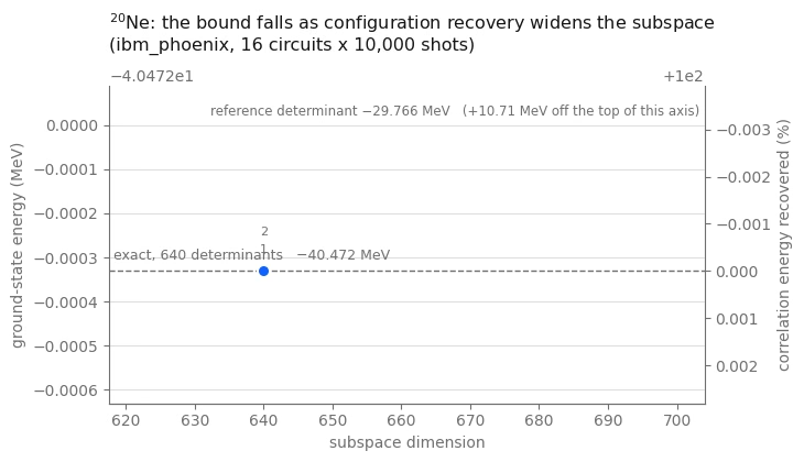
Large-scale hardware example
Scaling up changes only the inputs, so the next step is to combine the four stages into one function and run it twice, both times on a 40-qubit register in the shell above a core with the GXPF1 interaction [3].
The two runs illustrate different aspects of scaling:
- , two valence protons and two valence neutrons, has a 4,000-determinant basis. The register is 40 qubits, but the problem is still small enough to diagonalize exactly on a laptop, so you can compare the hardware result with an exact reference after increasing the register size.
- , four valence protons and four valence neutrons, has 1,963,461 symmetry-allowed determinants in the same 40 qubits. The tutorial's dense solver cannot diagonalize that full space, so the run returns a rigorous upper bound and the reference determinant it improves on.
Watch two quantities across the two runs. The fraction of the pool that fits inside the fixed gate
budget shrinks as the pool grows, and pack_ensemble reports how much is included. The
subspace stops being limited by sampling and starts being limited by MAX_DIMENSION, the largest
matrix the dense classical solver here builds. At this scale, a production
calculation would use a selected configuration interaction (selected-CI) solver.
Combine steps 1–4
The following function calls the same stages as the walkthrough, in the same order.
def sqd_run(snt_file, n_protons, n_neutrons, name, exact=True):
    """The whole workflow for one nucleus.  Returns a record of every stage."""
    # -------------------------Step 1-------------------------
    ms = read_snt(DATA / snt_file, n_protons, n_neutrons)
    sp = m_scheme_states(ms)
    inter = Interaction(ms, sp)
    if sum(1 for s in sp if s.tz == -1) * 2 != len(sp):
        raise ValueError(
            f"{name}: post-selection needs equal proton and neutron state counts"
        )
    reference = reference_determinant(sp, inter, n_protons, n_neutrons)
    e_ref = matrix_element(inter, reference, reference)

    raw = excitation_pool(sp, reference)
    ranked = rank_pool(
        inter, reference, [op for op in raw if conserves_symmetry(sp, op)]
    )
    print(
        f"{name}: {len(sp)} qubits, {n_protons}p + {n_neutrons}n, A = {ms.mass_number}"
    )
    print(
        f"  2p2h pool {len(raw)} raw -> {len(ranked)} symmetry-allowed; "
        f"reference energy {e_ref:.6f} MeV"
    )

    # -------------------------Step 2-------------------------
    costs = excitation_costs(len(sp), ranked, costing_manager)
    circuits, bins, isa = pack_to_budget(
        len(sp),
        reference,
        ranked,
        costs,
        DEPTH_BUDGET,
        N_CIRCUITS,
        pass_manager,
    )
    packed = sum(len(b) for b in bins)
    worst = max(two_qubit_depth(c) for c in isa)
    worst_count = max(two_qubit_count(c) for c in isa)
    print(
        f"  packed {packed} of {len(ranked)} excitations; worst circuit two-qubit depth "
        f"{worst}, {worst_count} two-qubit gates"
    )

    # -------------------------Step 3-------------------------
    # a unique tag per run, so the jobs are findable later
    bit_arrays = sample(isa, SHOTS, JOB_TAGS + [name])
    matrix, probabilities, shots = pool_samples(bit_arrays, sp)
    survival = float(
        probabilities[
            (matrix[:, len(sp) // 2 :].sum(axis=1) == n_protons)
            & (matrix[:, : len(sp) // 2].sum(axis=1) == n_neutrons)
        ].sum()
    )
    print(
        f"  {shots:,} shots -> {len(matrix):,} distinct bitstrings, "
        f"{survival:.1%} of shots with the right nucleon numbers"
    )
    if survival == 0.0:
        raise RuntimeError(
            f"{name}: no shot carried the right nucleon numbers"
        )

    # -------------------------Step 4-------------------------
    result = recovery_loop(
        inter,
        sp,
        matrix,
        probabilities,
        reference,
        n_protons,
        n_neutrons,
        max_iterations=4,
        max_dimension=MAX_DIMENSION,
        seed=42,
    )
    energy = result["energy"]

    full_dim = count_basis(sp, n_protons, n_neutrons)  # cheap, even when huge
    e_exact = None
    if exact:
        full = full_basis(sp, n_protons, n_neutrons)
        if len(full) != full_dim:
            raise AssertionError(
                f"{name}: counted {full_dim} determinants but enumerated "
                f"{len(full)}"
            )
        e_exact, _ = ground_state(inter, full)

    print(f"  reference {e_ref:11.6f} MeV     pooled SQD {energy:11.6f} MeV")
    if e_exact is not None:
        print(
            f"  exact     {e_exact:11.6f} MeV  (dimension {full_dim})  ->  "
            f"{100 * (energy - e_ref) / (e_exact - e_ref):.1f}% of the correlation energy"
        )
        if energy < e_exact - 1e-7:
            raise AssertionError(
                f"{name}: pooled SQD bound is below the exact energy"
            )
    else:
        print(
            f"  no exact reference: the symmetry-allowed basis is {full_dim:,} determinants"
        )
        print(
            f"  the bound captures {energy - e_ref:.6f} MeV of correlation energy"
        )
    print()

    return dict(
        name=name,
        qubits=len(sp),
        pool=len(ranked),
        packed=packed,
        two_qubit=worst,
        two_qubit_gates=worst_count,
        shots=shots,
        distinct=len(matrix),
        survival=survival,
        dimension=len(result["basis"]),
        full_dim=full_dim,
        e_ref=e_ref,
        e_sqd=energy,
        e_exact=e_exact,
        history=result["history"],
        # the subspace and its eigenvector cannot be reconstructed from the summary --
        # they depend on the sampled shots -- so keep them for the scaling analysis
        interaction=inter,
        states=sp,
        reference=reference,
        ranked=ranked,
        basis=result["basis"],
        vector=result["vector"],
    )

pretty = {"20Ne": "$^{20}$Ne", "44Ti": "$^{44}$Ti", "48Cr": "$^{48}$Cr"}

small_scale = dict(
    name="20Ne",
    qubits=len(sp_sd),
    pool=len(ranked_sd),
    packed=PACKED_SD,
    two_qubit=worst_sd,
    two_qubit_gates=worst_count_sd,
    shots=shots_sd,
    distinct=len(matrix_sd),
    survival=shot_survival_sd,
    dimension=len(result_sd["basis"]),
    full_dim=len(basis_exact_sd),
    e_ref=E_REF_SD,
    e_sqd=E_SQD_SD,
    e_exact=E_EXACT_SD,
    history=result_sd["history"],
    interaction=inter_sd,
    states=sp_sd,
    reference=occ_sd,
    ranked=ranked_sd,
    basis=result_sd["basis"],
    vector=result_sd["vector"],
)
: the same workflow on a 40-qubit register
The shell above has four orbitals per species and 20 magnetic substates each, so the register is 40 qubits. Two valence protons and two valence neutrons make , with 4,000 symmetry-allowed determinants — about six times the basis, using 40 qubits instead of 24.
This is the larger of the two examples that the notebook can solve exactly, so you can compare the hardware result with an exact reference.
large_scale_verified = sqd_run("gxpf1.snt", 2, 2, "44Ti", exact=True)
44Ti: 40 qubits, 2p + 2n, A = 44
  2p2h pool 1602 raw -> 174 symmetry-allowed; reference energy -44.309387 MeV
  packed 96 of 174 excitations; worst circuit two-qubit depth 272, 285 two-qubit gates
job dap31a02fm4c73f67dp0: 16 circuits x 10,000 shots on ibm_phoenix
  160,000 shots -> 48,170 distinct bitstrings, 18.6% of shots with the right nucleon numbers
  iteration 1: 187 proton x 189 neutron halves -> dimension 3891, E = -47.849086 MeV
  iteration 2: 190 proton x 190 neutron halves -> dimension 4000, E = -47.876666 MeV
  iteration 3: 190 proton x 190 neutron halves -> dimension 4000, E = -47.876666 MeV
  reference  -44.309387 MeV     pooled SQD  -47.876666 MeV
  exact      -47.876666 MeV  (dimension 4000)  ->  100.0% of the correlation energy
: beyond the tutorial's exact-diagonalization capacity
Adding two protons and two neutrons uses the same 40-qubit register (4, 4 for
) and increases the basis size by a factor of about 491, to 1,963,461 symmetry-allowed determinants. That
matrix is far beyond anything this tutorial will build, so exact=False: there is no exact reference energy,
only the variational bound and the reference determinant it improves on.
Two things change at this scale, and both are visible in the printout. The pool grows to several
hundred allowed excitations, so the fixed gate budget now covers a minority of it rather than all of
it. Also, the product subspace the samples span is larger than MAX_DIMENSION, so the dense solver
truncates it by sampled weight. The bound remains rigorous but can be less accurate than a bound
computed from all the sampled configurations. A production calculation would retain the samples
and use a solver that supports a larger subspace.
large_scale_unverified = sqd_run("gxpf1.snt", 4, 4, "48Cr", exact=False)
48Cr: 40 qubits, 4p + 4n, A = 48
  2p2h pool 5536 raw -> 582 symmetry-allowed; reference energy -93.041237 MeV
  packed 96 of 582 excitations; worst circuit two-qubit depth 224, 279 two-qubit gates
job dap32a02fm4c73f67eog: 16 circuits x 10,000 shots on ibm_phoenix
  160,000 shots -> 55,436 distinct bitstrings, 18.6% of shots with the right nucleon numbers
  iteration 1: 223 proton x 223 neutron halves -> dimension 3977, E = -96.481598 MeV
  iteration 2: 223 proton x 223 neutron halves -> dimension 3977, E = -96.481598 MeV
  reference  -93.041237 MeV     pooled SQD  -96.481598 MeV
  no exact reference: the symmetry-allowed basis is 1,963,461 determinants
  the bound captures -3.440361 MeV of correlation energy
Evaluate a result without an exact reference
The run has no exact reference within this tutorial. Use the existing samples to assess convergence and compare with the classical selection baseline, without additional QPU time or full-space diagonalization.
Is it converged? Reorder the retained determinants by their weight in the converged eigenvector
and the subspaces become nested, so diagonalizing the leading block for a ladder of
traces the bound's descent across two decades of subspace size. If it is still falling steeply at the
largest , the classical solver's dimension cap is the binding constraint and MAX_DIMENSION is the
parameter to increase. If it has flattened, adding more of the retained determinants offers little improvement;
further progress may require sampling additional configurations. The
Hamiltonian is built once at full size and every rung is a principal block of it, so the whole
sweep costs one matrix build rather than one per rung.
How does quantum sampling compare with classical selection? Compare with a subspace of the same size chosen by the classical selection procedure: take the pool ranked by perturbation theory in score order, grow the product subspace to the same dimension, and diagonalize that instead. Both curves are rigorous upper bounds on the same Hamiltonian, so whichever sits lower at equal dimension picked the better determinants. This comparison decides whether hardware sampling improves the energy estimate relative to this classical baseline.
This subspace is not selected for excited states. Configuration recovery steers the subspace using ground-state occupancies, so the higher eigenvalues are much further from converged than the lowest one, and the first excitation energy comes out well above the measured . Reaching excited states properly needs a subspace selected for them.
def subspace_scaling(
    inter, basis, vector, points=18, smallest=32, largest=None
):
    """Nested Rayleigh-Ritz sweep: the lowest eigenvalue of the leading d x d block, for a ladder of d.

    Reordering the basis by descending weight in the converged eigenvector makes every subspace in
    the ladder a subset of the next, so the energies fall monotonically and each one is a valid
    variational bound.  H is built once at full size; each rung is a principal block.
    """
    order = np.argsort(-(np.abs(vector) ** 2))
    ordered = [basis[i] for i in order]
    weights = (np.abs(vector) ** 2)[order]
    if (
        largest is not None
    ):  # cap the ladder so two subspaces end at a common dimension
        ordered, weights = ordered[:largest], weights[:largest]
    H = subspace_hamiltonian(inter, ordered)
    dimensions = np.unique(
        np.geomspace(smallest, len(ordered), points).astype(int)
    )
    rows = [
        (
            int(d),
            float(
                eigh(H[:d, :d], eigvals_only=True, subset_by_index=[0, 0])[0]
            ),
        )
        for d in dimensions
    ]
    return rows, np.cumsum(weights)

def classical_selection(
    inter, sp, reference, ranked, target, n_protons, n_neutrons
):
    """The subspace classical perturbative ranking would pick, grown to `target` dimension.

    Same product construction as the sampled subspace, and the same truncation discipline -- half
    configurations are offered to `grow_subspace` in order of importance and it takes as many as
    fit.  The only difference from the sampled path is where the ordering comes from: PT2 score
    here, measured sampling weight there.  So the comparison isolates *which determinants got
    chosen* and nothing else.

    Truncating by any other rule would not be a fair baseline.  Slicing an arbitrarily ordered
    list, for instance, keeps determinants by accident rather than by importance and makes the
    classical subspace look worse than classical selection really is.
    """
    p_ref = tuple(i for i in reference if sp[i].tz == -1)
    n_ref = tuple(i for i in reference if sp[i].tz == +1)
    reached = {reference}
    proton_order, neutron_order = [p_ref], [n_ref]
    seen_p, seen_n = {p_ref}, {n_ref}
    product_budget = 4 * target

    for op, _, _ in ranked:  # ranked is already in descending PT2 score
        h1, h2, v1, v2 = op
        fresh = {
            tuple(sorted(set(d) - {h1, h2} | {v1, v2}))
            for d in reached
            if {h1, h2} <= set(d) and not {v1, v2} & set(d)
        }
        reached |= fresh
        for det in fresh:  # first appearance fixes a half's rank
            half_p = tuple(i for i in det if sp[i].tz == -1)
            half_n = tuple(i for i in det if sp[i].tz == +1)
            if half_p not in seen_p:
                seen_p.add(half_p)
                proton_order.append(half_p)
            if half_n not in seen_n:
                seen_n.add(half_n)
                neutron_order.append(half_n)
        if len(proton_order) * len(neutron_order) > product_budget:
            # Half-configuration products over-count the subspace, because only the
            # symmetry-allowed ones survive `product_subspace`.  Stopping on the product
            # count alone can therefore leave the basis far short of `target`, so check
            # the dimension actually realized and widen the budget if it falls short.
            trial, _, _ = grow_subspace(
                sp,
                [p_ref],
                [n_ref],
                proton_order,
                neutron_order,
                n_protons,
                n_neutrons,
                max_dimension=target,
            )
            if len(trial) >= target:
                break
            product_budget *= 2

    basis, _, _ = grow_subspace(
        sp,
        [p_ref],
        [n_ref],
        proton_order,
        neutron_order,
        n_protons,
        n_neutrons,
        max_dimension=target,
    )
    return basis

run = large_scale_unverified
if "basis" not in run:
    raise RuntimeError(
        "this cell needs the subspace and eigenvector that sqd_run now returns; "
        "re-run the sqd_run definition and the 48Cr cell"
    )

print(
    f"{run['name']}: sweeping nested subspaces of the sampled basis "
    f"(dimension {run['dimension']})"
)
sampled_rows, cumulative = subspace_scaling(
    run["interaction"], run["basis"], run["vector"]
)

print(
    f"{run['name']}: building the classically selected subspace at the same dimension"
)
classical_basis = classical_selection(
    run["interaction"],
    run["states"],
    run["reference"],
    run["ranked"],
    run["dimension"],
    4,
    4,
)
# Both subspaces must be scored at the same dimension.  Symmetry filtering can still leave
# the classical construction short of the target when the ranked pool runs out, so take the
# dimension both actually reach, cap both ladders there, and verify they agree.
common_dim = min(sampled_rows[-1][0], len(classical_basis))
if common_dim < sampled_rows[-1][0]:
    sampled_rows, _ = subspace_scaling(
        run["interaction"], run["basis"], run["vector"], largest=common_dim
    )
classical_rows, _ = subspace_scaling(
    run["interaction"],
    classical_basis,
    ground_state(run["interaction"], classical_basis)[1],
    largest=common_dim,
)
if sampled_rows[-1][0] != classical_rows[-1][0]:
    raise RuntimeError(
        f"comparison dimensions differ: sampled {sampled_rows[-1][0]}, "
        f"classical {classical_rows[-1][0]}"
    )

advantage = sampled_rows[-1][1] - classical_rows[-1][1]
direction = "lower" if advantage < 0 else "higher"
verdict = "beats" if advantage < 0 else "does not beat"
descent = next(
    e for d, e in reversed(sampled_rows) if d <= sampled_rows[-1][0] / 2
)
for fraction in (0.90, 0.99):
    count = int(np.searchsorted(cumulative, fraction) + 1)
    print(
        f"  {fraction:.0%} of the eigenvector norm sits on {count} determinants "
        f"({count / run['full_dim']:.1e} of the {run['full_dim']:,}-determinant space)"
    )
print(
    f"  bound still falling {1000 * (sampled_rows[-1][1] - descent):+.1f} keV "
    f"over the last doubling of dimension"
)
print(
    f"  sampled {sampled_rows[-1][1]:.6f} MeV vs classically selected "
    f"{classical_rows[-1][1]:.6f} MeV at a verified common dimension of "
    f"{classical_rows[-1][0]:,}"
)
print(
    f"  -> the sampled subspace is {abs(advantage) * 1000:.0f} keV {direction}"
)
48Cr: sweeping nested subspaces of the sampled basis (dimension 3977)
48Cr: building the classically selected subspace at the same dimension
  90% of the eigenvector norm sits on 107 determinants (5.4e-05 of the 1,963,461-determinant space)
  99% of the eigenvector norm sits on 593 determinants (3.0e-04 of the 1,963,461-determinant space)
  bound still falling -15.6 keV over the last doubling of dimension
  sampled -96.481598 MeV vs classically selected -95.314510 MeV at a verified common dimension of 3,957
  -> the sampled subspace is 1167 keV lower
fig, axes = plt.subplots(1, 2, figsize=(11.2, 4.0), facecolor=SURFACE)

# left: two nested convergence curves on the same axes
ax = axes[0]
ax.set_facecolor(SURFACE)
ax.plot(
    [d for d, _ in sampled_rows],
    [e for _, e in sampled_rows],
    "-o",
    color=SERIES,
    linewidth=2,
    markersize=5,
    markeredgecolor=SURFACE,
    markeredgewidth=1,
    zorder=4,
    label="sampled on the QPU",
)
ax.plot(
    [d for d, _ in classical_rows],
    [e for _, e in classical_rows],
    "--s",
    color=MUTED,
    linewidth=1.6,
    markersize=4,
    markeredgecolor=SURFACE,
    markeredgewidth=1,
    zorder=3,
    label="classically selected, same size",
)
ax.axhline(run["e_ref"], color=RULE, linestyle=":", linewidth=1.2, zorder=1)
ax.annotate(
    f"reference determinant {run['e_ref']:.2f} MeV".replace("-", "\u2212"),
    xy=(sampled_rows[-1][0], run["e_ref"]),
    xytext=(-2, 4),
    textcoords="offset points",
    ha="right",
    va="bottom",
    color=MUTED,
    fontsize=8,
)

# mark the gap between the two curves at the largest dimension, not either curve alone
edge = sampled_rows[-1][0]
ax.plot(
    [edge, edge],
    [classical_rows[-1][1], sampled_rows[-1][1]],
    "-",
    color=SERIES,
    linewidth=1.0,
    alpha=0.7,
    zorder=2,
)
ax.annotate(
    f"{abs(advantage) * 1000:.0f} keV {direction}\nat equal dimension",
    xy=(edge, 0.5 * (classical_rows[-1][1] + sampled_rows[-1][1])),
    xytext=(-8, 0),
    textcoords="offset points",
    ha="right",
    va="center",
    color=SERIES,
    fontsize=8.5,
)

ax.set_xscale("log")
ax.set_xlim(sampled_rows[0][0] * 0.75, edge * 1.5)
ax.set_xlabel("subspace dimension", color=MUTED)
ax.set_ylabel("variational upper bound (MeV)", color=MUTED)
ax.set_title(
    f"{pretty[run['name']]}: the bound, and the subspace it {verdict}",
    color=INK,
    fontsize=11,
    loc="left",
    pad=10,
)
legend = ax.legend(frameon=False, fontsize=8.5, loc="lower left")
for text in legend.get_texts():
    text.set_color(MUTED)

# right: why a few thousand determinants can bound two million
ax = axes[1]
ax.set_facecolor(SURFACE)
ranks = np.arange(1, len(cumulative) + 1)
ax.plot(ranks, 100 * cumulative, "-", color=DEEP, linewidth=2, zorder=3)
for fraction, style, label_y in ((0.90, ":", 46), (0.99, "--", 24)):
    count = int(np.searchsorted(cumulative, fraction) + 1)
    ax.axvline(count, color=MUTED, linestyle=style, linewidth=1, zorder=1)
    ax.annotate(
        f"{fraction:.0%} of the norm\non {count} determinants",
        xy=(count, label_y),
        xytext=(7, 0),
        textcoords="offset points",
        ha="left",
        va="center",
        color=MUTED,
        fontsize=8.5,
    )
ax.set_xscale("log")
ax.set_xlim(0.8, len(cumulative) * 2.6)
ax.set_ylim(0, 104)
ax.set_xlabel("determinants, ordered by weight", color=MUTED)
ax.set_ylabel("cumulative share of the eigenvector (%)", color=MUTED)
ax.set_title(
    f"Sparsity: {run['full_dim']:,} determinants in the sector",
    color=INK,
    fontsize=11,
    loc="left",
    pad=10,
)

for ax in axes:
    ax.grid(axis="y", color=RULE, alpha=0.55)
    ax.tick_params(colors=MUTED, labelsize=8.5)
    for side in ("top", "right"):
        ax.spines[side].set_visible(False)
    for side in ("bottom", "left"):
        ax.spines[side].set_color(MUTED)
fig.tight_layout()
plt.show()
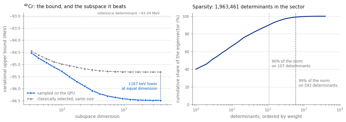
Compare the three runs
Absolute energies are not comparable across different nuclei and different interactions, so focus on the fraction of the correlation energy recovered across runs, where an exact reference is available. Also compare circuit depth and the fraction of discarded shots.
runs = [small_scale, large_scale_verified, large_scale_unverified]

print(
    f"{'run':>6}  {'qubits':>6}  {'pool':>9}  {'2q depth':>8}  {'2q gates':>8}  "
    f"{'shots kept':>10}  {'dim':>6}  {'of':>9}  {'% corr':>7}"
)
for r in runs:
    fraction = (
        "--"
        if r["e_exact"] is None
        else f"{100 * (r['e_sqd'] - r['e_ref']) / (r['e_exact'] - r['e_ref']):.1f}%"
    )
    coverage = "{}/{}".format(r["packed"], r["pool"])
    print(
        f"{r['name']:>6}  {r['qubits']:>6}  {coverage:>9}  "
        f"{r['two_qubit']:>8}  {r['two_qubit_gates']:>8}  {r['survival']:>9.1%}  "
        f"{r['dimension']:>6}  {(r['full_dim'] or 0):>9,}  {fraction:>7}"
    )

print()
for r in runs:
    exact = (
        f"exact {r['e_exact']:11.6f}"
        if r["e_exact"] is not None
        else "exact  unavailable"
    )
    print(
        f"{r['name']:>6}   reference {r['e_ref']:11.6f}   pooled SQD {r['e_sqd']:11.6f}   {exact} MeV"
    )
run  qubits       pool  2q depth  2q gates  shots kept     dim         of   % corr
  20Ne      24      78/78       228       234      31.5%     640        640   100.0%
  44Ti      40     96/174       272       285      18.6%    4000      4,000   100.0%
  48Cr      40     96/582       224       279      18.6%    3977  1,963,461       --

  20Ne   reference  -29.765549   pooled SQD  -40.472331   exact  -40.472331 MeV
  44Ti   reference  -44.309387   pooled SQD  -47.876666   exact  -47.876666 MeV
  48Cr   reference  -93.041237   pooled SQD  -96.481598   exact  unavailable MeV
# Left: how much of the correlation energy was recovered, where the exact answer is known.
# Right: the bound itself for the run that has nothing to score against.
scored = [r for r in runs if r["e_exact"] is not None]

fig, ax = plt.subplots(figsize=(6.4, 3.9), facecolor=SURFACE)
ax.set_facecolor(SURFACE)
labels = [
    f"{pretty[r['name']]}\n{r['qubits']} qubits\n{r['full_dim']:,} determinants"
    for r in scored
]
fractions = [
    100 * (r["e_sqd"] - r["e_ref"]) / (r["e_exact"] - r["e_ref"])
    for r in scored
]
shades = [SERIES, DEEP, PURPLE]
bars = ax.bar(
    labels, fractions, width=0.46, color=shades[: len(scored)], zorder=3
)
for bar, fraction, r in zip(bars, fractions, scored):
    ax.annotate(
        f"{fraction:.1f}%",
        xy=(bar.get_x() + bar.get_width() / 2, fraction),
        xytext=(0, 5),
        textcoords="offset points",
        ha="center",
        va="bottom",
        color=INK,
        fontsize=10,
    )
    ax.annotate(
        f"dim {r['dimension']:,}",
        xy=(bar.get_x() + bar.get_width() / 2, 3),
        ha="center",
        va="bottom",
        color=SURFACE,
        fontsize=8.5,
    )
ax.axhline(100, color=MUTED, linestyle="--", linewidth=1, zorder=1)
ax.annotate(
    "exact diagonalization",
    xy=(-0.45, 100),
    xytext=(0, 4),
    textcoords="offset points",
    ha="left",
    va="bottom",
    color=MUTED,
    fontsize=8.5,
)
ax.set_ylim(0, 118)
ax.set_ylabel("correlation energy recovered (%)", color=MUTED)
ax.set_title(
    f"Where the exact answer is known ({backend.name})",
    color=INK,
    fontsize=11,
    loc="left",
    pad=10,
)
ax.grid(axis="y", color=RULE, alpha=0.55)
ax.tick_params(colors=MUTED, labelsize=8.5)
for side in ("top", "right"):
    ax.spines[side].set_visible(False)
for side in ("bottom", "left"):
    ax.spines[side].set_color(MUTED)
fig.tight_layout()
plt.show()

# the same convergence view as the walkthrough, for the run with no exact reference
convergence_plot(
    large_scale_unverified["history"],
    large_scale_unverified["e_ref"],
    None,
    f"{pretty[large_scale_unverified['name']]}: "
    f"{large_scale_unverified['full_dim']:,} determinants, no exact answer to score against\n"
    f"({backend.name}, {N_CIRCUITS} circuits x {SHOTS:,} shots)",
    colour=DEEP,
)
plt.show()

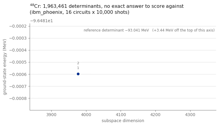
Summary
One workflow, unchanged apart from its inputs, ran on a QPU at three problem sizes: a 24-qubit problem you can check exactly, a 40-qubit problem you can still check exactly, and a 40-qubit problem with nearly two million basis states beyond this tutorial's exact-diagonalization capacity.
The three runs illustrate the following points:
- The quantum step only has to propose determinants. The circuit is fixed, seeded from second-order perturbation theory, and never optimized. Nothing in the workflow needs its amplitudes to be accurate, only its support to be useful. Classical diagonalization in the selected subspace gives a variational upper bound, although the bound varies with the sampled configurations.
- Qubit excitations reduce circuit depth. Because only the support matters, the fermionic excitation blocks can be replaced by qubit excitations, whose cost does not grow with the distance between the orbitals they connect. Step 2 measured the saving on the actual backend, which is the difference between a circuit that fits comfortably inside coherence and one that does not.
- Configuration recovery reuses noisy samples. Every shot with the wrong proton or neutron number is repaired against the current occupancy estimate rather than discarded, and each repaired half-configuration can add configurations to the subspace. Widening a variational subspace cannot raise its lowest eigenvalue. This tutorial demonstrates configuration recovery using hardware samples.
- The binding constraint moves as you scale. At 24 qubits the ansatz could reach the exact answer, and only sampling stood in the way. At 40 qubits with four valence nucleons per species, the gate budget covers a minority of the pool and the dense classical solver caps the subspace. Knowing which of the three is limiting you is the practical skill this workflow teaches.
Next steps
Explore these related resources:
- Sample-based quantum diagonalization of a chemistry Hamiltonian: the same algorithm applied to electronic structure, using the SQD addon's selected-CI solver.
- SQD addon documentation: post-selection, subsampling, and configuration-recovery utilities.
- Quantum diagonalization algorithms: a full course on subspace diagonalization, including Krylov variants.
- Introduction to transpilation: the pass-manager options that matter when a circuit is dominated by two-qubit gates.
- Execution modes: explore batch mode for scheduling independent jobs.
Extensions to consider
- Replace the dense solver.
MAX_DIMENSIONis the ceiling on everything at the scale, andnp.linalg.eighon a dense matrix is why. Building the same projected Hamiltonian as a sparse matrix and using an iterative eigensolver such asscipy.sparse.linalg.eigsh, or a Davidson or selected-CI solver designed for nuclear two-body interactions, could support larger subspaces. The practical limit depends on matrix sparsity, available memory, and solver convergence, and this tutorial does not benchmark that extension. The SQD addon'sqiskit_addon_sqd.fermion.solve_sciis not a drop-in substitute: it wraps an electronic-structure solver and expects one- and two-body integrals in that form, so the shared proton neutron product structure is not sufficient on its own. Using it would mean mapping the shell-model interaction of Equation (1) into those integrals and validating the result against the exact energies this notebook already computes. - Add batching and subsampling. The published pooled SQD workflow diagonalizes several independent subsamples per iteration and keeps the best. This tutorial uses one batch per iteration, which is harmless for the variational bound but does not provide the variance information that indicates whether more shots would help.
- Excited states and other sectors. The higher eigenvalues of each subspace Hamiltonian are upper bounds on excited states in the same symmetry sector, and running at reaches other sectors. The check in Step 1 is already half of this calculation.
- A cross-shell model space. Parity is automatically satisfied inside a single major shell, which is why it does no work here. An - space mixes parities, making parity a genuine fourth constraint, one that neither SQD's Hamming-weight repair nor the product construction would catch on its own.
- Odd-mass nuclei.
reference_determinantrequires an even valence count in each species, because a time-reversed paired filling is what forces . An odd nucleus needs a half-integer target and an unpaired reference.
Appendix
This section explains the reasoning behind the helpers introduced in the Setup section.
Why the mass-dependence rescaling is not optional
Empirical shell-model interactions are fitted at one mass and applied across a chain of isotopes, with
the two-body matrix elements scaled as . Both interaction files carry
, with for the USD family and for GXPF1. On the two-body header
line of a .snt file, those two numbers sit where an oscillator frequency and a core energy would
plausibly go, which makes them easy to misread; reading the exponent as a constant core energy adds a
spurious offset to every diagonal element and drops the rescaling, changing the correlation energy by
a few percent. The symmetry check in Step 1 does not by itself verify the energy scale. Comparing
the excitation energy, measured in MeV, with experiment provides an additional check on the
mass-dependent rescaling. An excitation energy is a difference between levels, so it does not
detect a constant offset applied to all energies.
Why the reference is found by search rather than by filling
The obvious reference is the determinant that fills the lowest single-particle energies. It is not the lowest-energy determinant, because the diagonal of Equation (1) includes the two-body term , and the pairing interaction strongly prefers occupying time-reversed partners in the largest available . In the shell that is the difference between the pair and the pair of , and it is worth about 1 MeV; in the shell, it is worth closer to 2. Because the reference energy defines the zero of the "correlation energy recovered" metric, a poor choice inflates that metric and gives a less accurate starting point.
Restricting to paired fillings makes exhaustive search inexpensive, with candidates per species (a few thousand at most), and ensures . In every case in this tutorial that can be checked against a full enumeration, the search returns the global lowest-diagonal determinant, which is also the single largest component of the exact ground state.
Why the first-order amplitude, not the exact two-level angle
Diagonalizing the Hamiltonian in the space gives the mixing angle ; it might be tempting to call that the correct choice for an isolated pair of levels. In this ansatz, several dozen excitation blocks act in sequence on the same reference, so optimizing each block separately does not necessarily optimize the composite circuit.
The circuit’s role determines the choice of angle. Since for every real , the exact angle is always smaller in magnitude than the first-order amplitude , and therefore always leaves more amplitude on the reference determinant. A circuit that keeps more amplitude on the reference returns the reference more often and distinct excited determinants less often. For pooled SQD, the useful output of a shot is a determinant the classical step has not seen yet, which motivates using the larger angle in this tutorial. Neither angle needs to be accurate, because the classical diagonalization discards the circuit's amplitudes entirely and re-derives its own.
Why pooled SQD can use qubit excitations
The fermionic excitation maps under Jordan-Wigner to eight Pauli strings, each carrying operators on every qubit between the outermost indices. Those strings encode the fermionic sign, and their cost grows with the span, which for a proton-neutron excitation is the whole register.
Deleting them gives the qubit-excitation operator of Yordanov et al. [5]. It is a different operator: the state it prepares differs from the fermionic one in the signs of its amplitudes, and the two sampling distributions can differ substantially. What it does not change is which determinants have nonzero amplitude, because each block still rotates within the same two-dimensional space for every determinant it acts on, and it still conserves both nucleon numbers, , and parity exactly. The reachable set of determinants is therefore identical, and the reachable set is the only thing pooled SQD uses; the classical diagonalization assigns its own amplitudes regardless. Step 2 verifies the identical-support claim on a real operator from the pool and measures what the substitution saves.
The limitation is that the sampling weights differ, so the two constructions will not discover determinants in the same order at finite shot count. Since the ranking that decides which excitations enter the circuits is classical and unchanged, and the classical step re-weights everything anyway, the difference in sampling weights is a tradeoff for reduced circuit depth.
Why belongs to the product stage
Post-selection and configuration recovery both act on Hamming weights: the number of protons in one
half of the register, and the number of neutrons in the other. is not of that form. It is a property of a proton configuration paired with a neutron configuration. A shot whose proton
half and neutron half each carry the right nucleon number contains two usable half-configurations even
when their values do not cancel, because the proton half at is perfectly good once it
is paired with a neutron half at . Filtering whole shots on total throws both halves
away, and imposing on the recombined products keeps them. The same argument explains why
recover_configurations needs no notion of to be useful in this case.
References
- J. Robledo-Moreno, M. Motta, H. Haas, et al., "Chemistry beyond the scale of exact diagonalization on a quantum-centric supercomputer", Science Advances 11, eadu9991 (2025). arXiv:2405.05068
- B. A. Brown and W. A. Richter, "New USD Hamiltonians for the sd shell", Physical Review C 74,
034315 (2006). The embedded
usda.sntfile carries the USDA parameters as tabulated by W. A. Richter, S. Mkhize and B. A. Brown, "sd-shell observables for the USDA and USDB Hamiltonians", Physical Review C 78, 064302 (2008). - M. Honma, T. Otsuka, B. A. Brown and T. Mizusaki, "Effective interaction for pf-shell nuclei", Physical Review C 65, 061301(R) (2002).
- B. Huron, J. P. Malrieu and P. Rancurel, "Iterative perturbation calculations of ground and excited state energies from multiconfigurational zeroth-order wavefunctions", The Journal of Chemical Physics 58, 5745 (1973).
- Y. S. Yordanov, D. R. M. Arvidsson-Shukur and C. H. W. Barnes, "Efficient quantum circuits for quantum computational chemistry", Physical Review A 102, 062612 (2020).
- National Nuclear Data Center, Evaluated Nuclear Structure Data File, Brookhaven National Laboratory. Source of the measured excitation energies quoted in Step 1.