Modern workflows

This course has covered a wide variety of methods for handling quantum noise and errors. We intentionally avoided some black-box solutions so that we could see how these methods work. Now we are ready to use these methods in their most modern form. Specifically, we explore some highly optimized error-handling tools that hide some of the complexity from us. We also explore Samplomatic and addons such as shaded lightcones (SLC), which give us very fine control over certain mitigation processes.

In this video, Dr. Chris Porter gives an overview of these modern tools. We plan to add example workflows to this lesson at a later date. However, this lesson already contains all the information that you need to use these tools and to pass the badging exam.

Overview

Early IBM Quantum primitives, such as Estimator and Sampler, exposed error mitigation through a small number of preset levels. Later releases provided more direct control over individual techniques, including choices of zero-noise extrapolation strategy, Pauli twirling configurations, and randomization parameters. However, these settings remained largely global, and applied uniformly across an entire circuit.

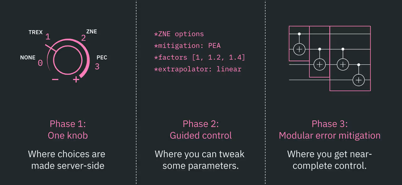
As quantum workloads become more sophisticated, developers increasingly need the ability to tailor execution and mitigation strategies to specific regions of a circuit. The following diagram outlines several key tools that this lesson discusses, and shows where they fit within a typical workflow.

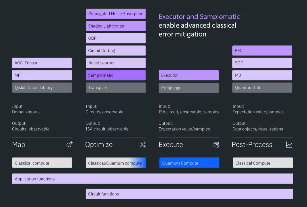
The directed execution model addresses the need for modular control over execution, and it integrates many of these tools.

Directed execution model

Rather than making implicit execution decisions, the directed execution model follows user-provided directives. This approach improves transparency and makes complex workflows easier to inspect and debug. Some key features of this model include:

• Per-layer configuration through labeled circuit regions
• Identification of unique and repeated layers for efficient noise learning
• Batched execution workflows
• Structured post-processing
• Close integration with addons such as shaded lightcones

The model is built around two key components:

• Samplomatic, which defines execution recipes
• Executor, which carries out those recipes and returns samples

Most workflows that use Executor can also be implemented with Sampler, because both ultimately produce samples. The key advantage of Executor is efficiency. Tasks such as generating twirling configurations are often much faster in the server-side near-time environment than on the client. Estimator and Sampler remain supported, and might still be the most convenient choice for many workloads.

Before execution, however, you must construct and prepare a circuit. Qiskit provides several addons that help with circuit generation, simulation, and optimization. For more information about any of the following tools, follow the links.

Build quantum circuits

For some applications or new approaches, users must determine how to map their problem to a quantum circuit. In many domains, however, Qiskit addons can automate important parts of this process.

Optimization mapper

Optimization mapper helps express classical optimization problems in forms that are suitable for quantum algorithms. Key functionality includes:

• Construct objective functions and constraints
• Convert problems into QUBO formulations
• Generate Hamiltonian or operator representations

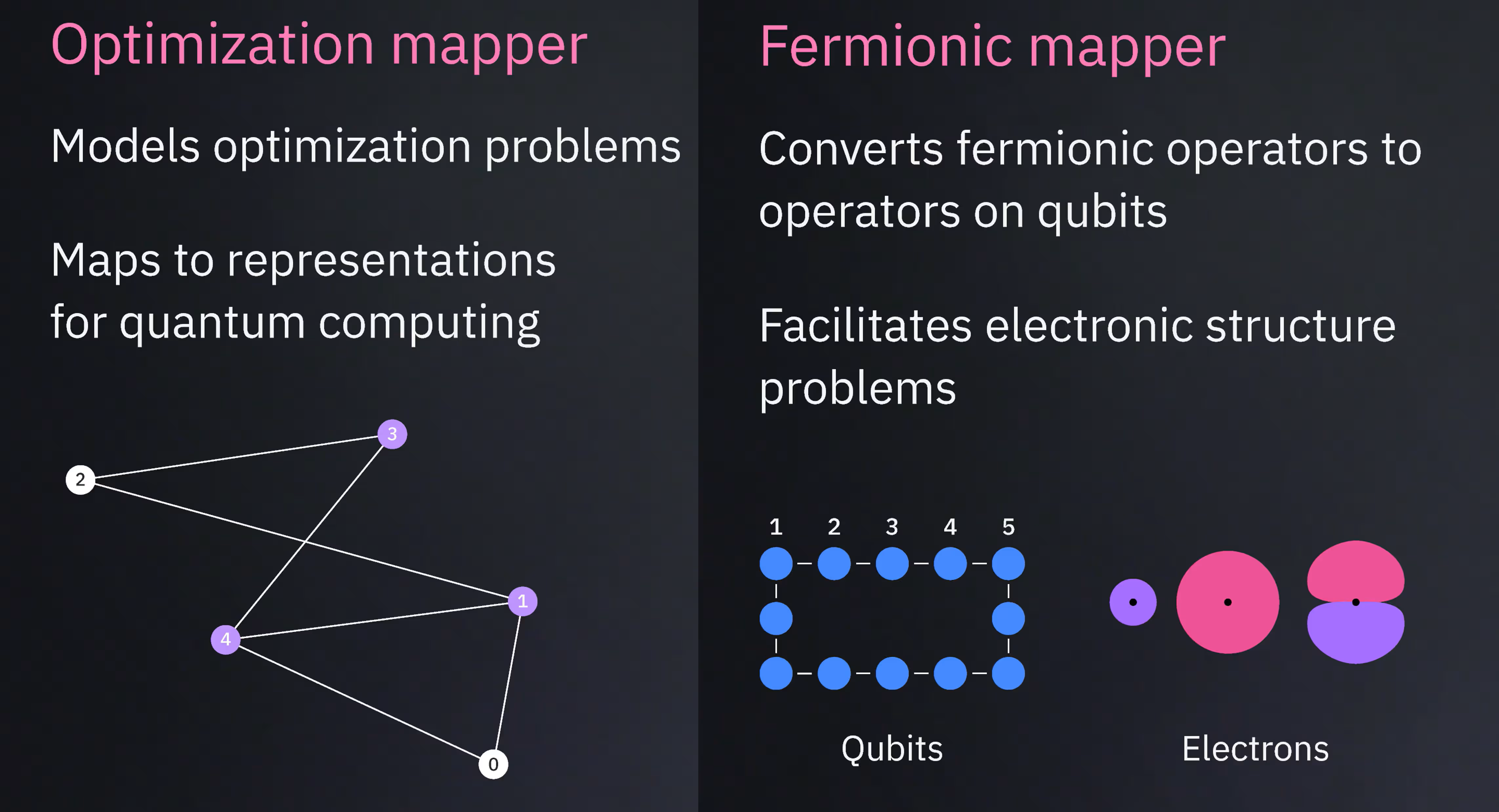
Fermionic mapper

Fermionic mapper converts fermionic operators into qubit operators that are suitable for quantum hardware. It supports mappings such as Jordan-Wigner, which converts operators on indistinguishable fermions to Pauli operators on distinguishable qubits, while preserving fermionic statistics. This addon is useful for quantum chemistry and materials science applications.

The previous two addons focus on the initial mapping of a problem structure to a quantum circuit. It is equally important, however, to efficiently map the time evolution of a process onto a quantum circuit, and to optimize a circuit by reducing its depth. The next few addons address these tasks.

Multi-product formulas (MPF)

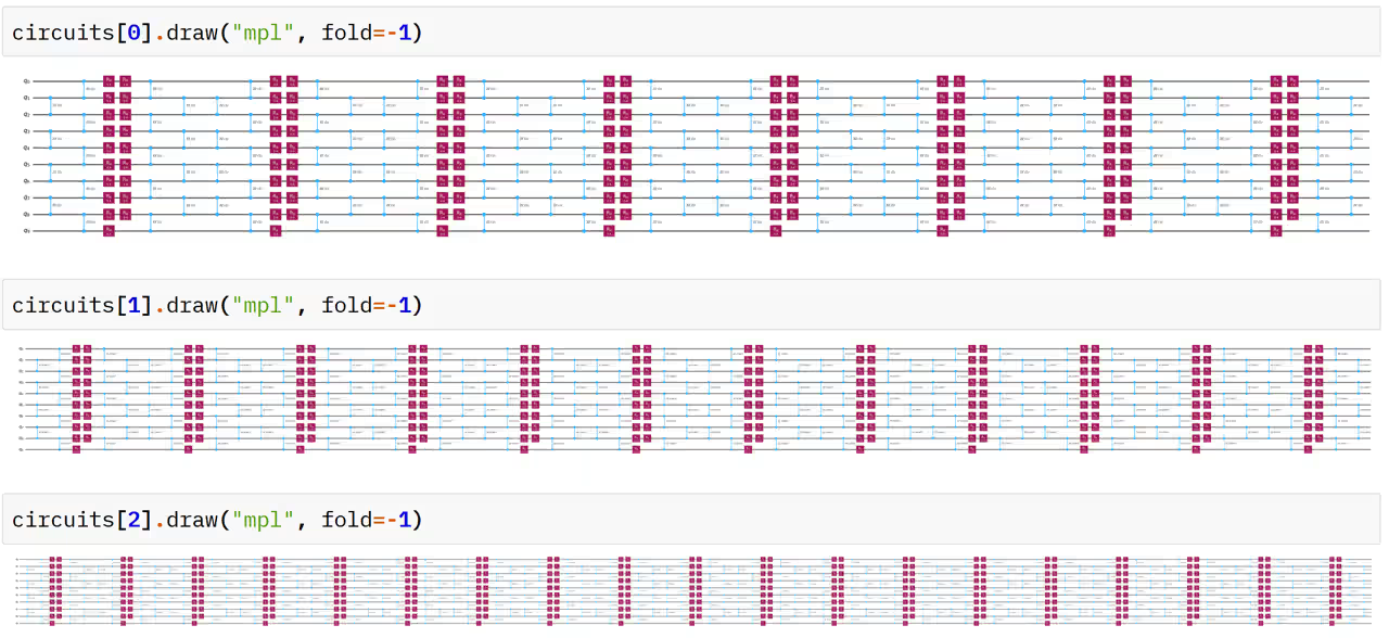
Multi-product formulas improve the accuracy of quantum time-evolution simulations by combining multiple approximations. Specifically, you create circuits with varying numbers of Trotter steps, so that you can use a weighted combination of the circuit results. For a given target accuracy, MPF can often use shallower circuits than standard Trotter methods. The cost is that you must run multiple circuits and combine their results classically.

AQC-Tensor

AQC-Tensor performs approximate quantum compilation using tensor-network methods. A common use case is to replace a portion of a deep circuit with a shallower variational approximation. The resulting circuit can achieve similar accuracy with significantly less depth.

Transpilation

You have already used transpilation many times in this course. You know that after an abstract circuit is constructed, it must be prepared for execution on hardware. However, we have not yet explored the multiple stages of transpilation in detail.

Key transpilation stages include:

• Layout: map logical qubits to physical qubits
• Translation: rewrite operations using the backend's native gate set
• Routing: insert and optimize SWAP operations required by hardware connectivity

These processes are interrelated. For example, the layout should minimize depth even after routing is taken into account. The layout should also avoid the most error-prone qubits and connections. These stages are often automated, but advanced users might choose to specify custom layouts or other constraints when needed.

To learn more about transpilation, see the Introduction to transpilation guide.

Check your understanding

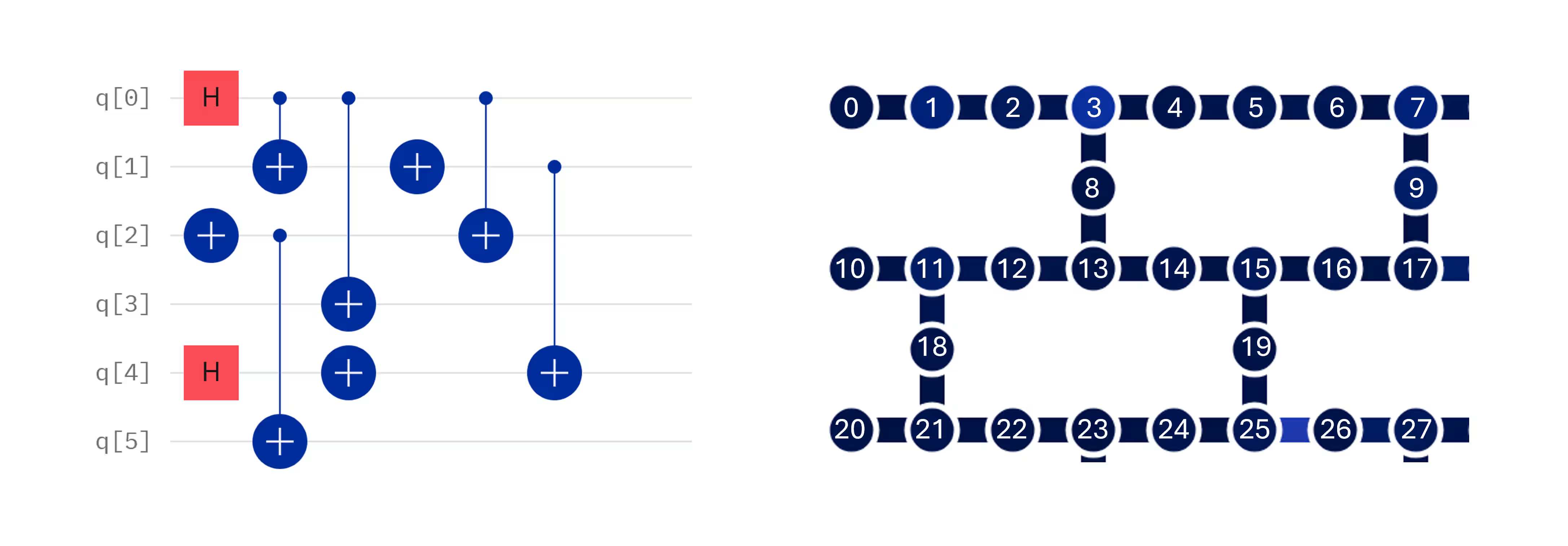
Look at the following quantum circuit, and assume that you need to run it on a quantum computer with a heavy-hex layout, part of which is shown. (a) Propose a mapping from the qubit numbers in the abstract circuit to the qubit numbers in the physical quantum computer that minimizes the number of SWAP gates required. (b) Is your choice unique, or might there be other equally good choices? (c) Even if your choice is the sole optimal layout for reducing SWAP gates, what are some reasons that the transpiler might choose a different mapping?

Answer

(a) There could be many correct answers, but note that only abstract qubit 0 has entangling (two-qubit) gates with three neighbors. All others participate in two-qubit operations with only two neighbors. This circuit can be mapped to a heavy-hex topology without any SWAP gates. Any layout that achieves this is acceptable. Using $\text{aq[0]}$ to refer to abstract qubit zero, and $\text{tq[0]}$ for transpiled qubit zero, one such layout is:

$$\begin{aligned} \text{aq[0]} & \rightarrow \text{tq[15],}\\ \text{aq[1]} & \rightarrow \text{tq[16],}\\ \text{aq[2]} & \rightarrow \text{tq[19],}\\ \text{aq[3]} & \rightarrow \text{tq[14],}\\ \text{aq[4]} & \rightarrow \text{tq[17],}\\ \text{aq[5]} & \rightarrow \text{tq[25]} \end{aligned}$$

(b) This layout is not unique. Many other layouts avoid SWAP gates altogether. Another example is:

$$\begin{aligned} \text{aq[0]} & \rightarrow \text{tq[3],}\\ \text{aq[1]} & \rightarrow \text{tq[4],}\\ \text{aq[2]} & \rightarrow \text{tq[8],}\\ \text{aq[3]} & \rightarrow \text{tq[2],}\\ \text{aq[4]} & \rightarrow \text{tq[5],}\\ \text{aq[5]} & \rightarrow \text{tq[13]} \end{aligned}$$

(c) Sometimes a specific qubit is more error-prone than most others on the chip. Also, some connections between qubits are more error-prone than others. The transpiler attempts to find a layout that avoids unnecessary SWAP gates, but that also uses the highest-fidelity qubits and connections available on the selected quantum computer.

Reduce the effects of noise and errors

Several Qiskit addons focus specifically on reducing the impact of noise and hardware imperfections.

Operator backpropagation and noise-aware circuit transformations

We have already discussed operator propagation in the context of coherent Pauli checks in error correction. However, operator propagation is useful more generally. There are two main ways to use the propagation of an operator through a quantum circuit: (1) absorb the last few layers of a quantum circuit into the observables being measured, and (2) take into account the likely effects of errors in the circuit, and compensate for them by measuring a different observable. The next two tools use these approaches.

Operator backpropagation

Operator backpropagation reduces circuit depth by absorbing gates from the end of a circuit into the measured observable. For example, consider the following circuit.

This circuit contains rotation and entangling layers that appear nontrivial, followed by a ladder of CNOT gates and a measurement of Z on qubit 5. This circuit has a two-qubit depth of 7. This depth is before transpilation. In practice, you typically apply backpropagation after transpilation, but this example is for teaching purposes only. Recall that there are rules for propagating an observable past a gate. In particular, when a CNOT gate has target $q_t$ and control $q_c$, a $Z_t$ observable on $q_t$ becomes $Z_c Z_t$ when propagated backward past the CNOT gate: $Z_t \rightarrow Z_c Z_t$. In this example circuit, if you propagate the observable $Z_5$ back through the entire ladder of CNOT gates, you get the observable $Z_5 Z_4 Z_3 Z_2 Z_1 Z_0$, or in standard Qiskit notation, simply $ZZZZZZ$. If we measure this observable instead of only $Z_5$, we can remove the entire ladder of CNOT gates, which reduces the two-qubit depth from 7 to 2. This observable still requires a measurement in only one basis on each qubit, so it does not increase the number of shots that we require. This is not always the case. Generally, more complicated observables require more shots, and sometimes more measurements in different bases.

The overall strategy of operator backpropagation includes the following steps:

• Shorten the executed circuit
• Replace the original observable with an expanded observable
• Trade circuit depth for increased sampling requirements

The previous circuit is an obvious example in which backpropagation is advantageous. In general, however, it is not easy to identify the circuits that benefit most from backpropagation. To decide when to use backpropagation, check how much depth you can remove from your circuit, and weigh that reduction against the increased sampling requirements.

Propagated noise absorption (PNA)

Propagated noise absorption is structurally similar to operator backpropagation. However, instead of propagating an operator back through the ideal gates in a circuit, PNA incorporates a learned noise model and propagates the effects of noise directly into the observable. PNA does the following:

• Learns noise behavior from the hardware
• Propagates the noise model through the circuit
• Produces a modified observable that compensates for gate noise

When the modified observable is measured on noisy hardware, the resulting expectation values better approximate the ideal noiseless result. PNA has two types of overhead. First, you must learn the noise model, which requires running additional circuits. Second, PNA can produce more complicated observables, which can increase sampling requirements.

Circuit cutting

Circuit cutting partitions a large circuit into smaller subcircuits that can run independently. You then make enough measurements to recombine the results. Circuit cutting does the following:

• Reduces hardware requirements
• Allows computations larger than available qubit counts (wider circuits)
• Helps address depth and connectivity limitations (deeper circuits)
• Reconstructs the original result through classical post-processing

Samplomatic

Many of the techniques in the previous sections complement other suppression and mitigation methods covered throughout this course, including:

• Dynamical decoupling
• Pauli twirling
• M3
• TREX
• Zero-noise extrapolation (ZNE)
• Probabilistic error cancellation (PEC)

In many workflows, you can apply different techniques to different regions of the same circuit. As we have seen, many of these techniques also come with quantum overhead. We therefore sometimes need fine, detailed control over noise learning, sampling, and the application of twirling sequences. These are some of the motivations behind Samplomatic.

Samplomatic is an open-source library that enables customized sampling, randomization, and error-mitigation workflows.

Its first task is to analyze a circuit and divide it into labeled regions, or boxes. These boxes serve two purposes:

• They visually partition the circuit.
• They create indexed regions that can be configured independently.

Users can attach annotations that describe how each box should be treated during execution. Examples include:

• Applying Pauli twirling to all boxes
• Applying twirling only to selected boxes
• Using different twirling groups in different regions
• Injecting learned noise into specific layers
• Customizing mitigation strategies at a fine-grained level

Samplomatic also identifies repeated boxed regions. Because identical layers typically exhibit similar noise characteristics, you only need to perform noise learning once for each unique layer.

Samplomatic outputs

Samplomatic produces two primary objects:

• Template circuit
• Samplex

The template circuit is a boxed, transpiled, parameterized circuit that is ready for execution. The samplex contains all the information that is required to generate and process circuit variants. Samplex contents include:

• Parameter values for parameterized circuits
• Randomization selections
• Sampling distributions
• Post-processing information
• Additional execution metadata

Formally, a samplex is a probability distribution over the parameters of a template circuit, together with auxiliary information that is required for execution and post-processing. An important practical advantage is that both the template circuit and the samplex are created locally on the client side. As a result, you can inspect, validate, and debug them before you use any hardware resources.

Samplomatic has many benefits, including fine-grained control of adaptive shot allocation and randomization. It also has logistical benefits, such as structured post-processing workflows. One of the most important benefits is the reuse of learned noise information across identical layers, which can save a significant amount of quantum computing time during noise learning.

Shaded lightcones

Before you decide where to apply expensive mitigation techniques, it is helpful to identify the regions of a circuit that matter most to the observable that is being measured. This need motivates the shaded lightcones addon. The idea of a lightcone comes from relativity, in which causal relationships are constrained by the finite speed at which information can travel.

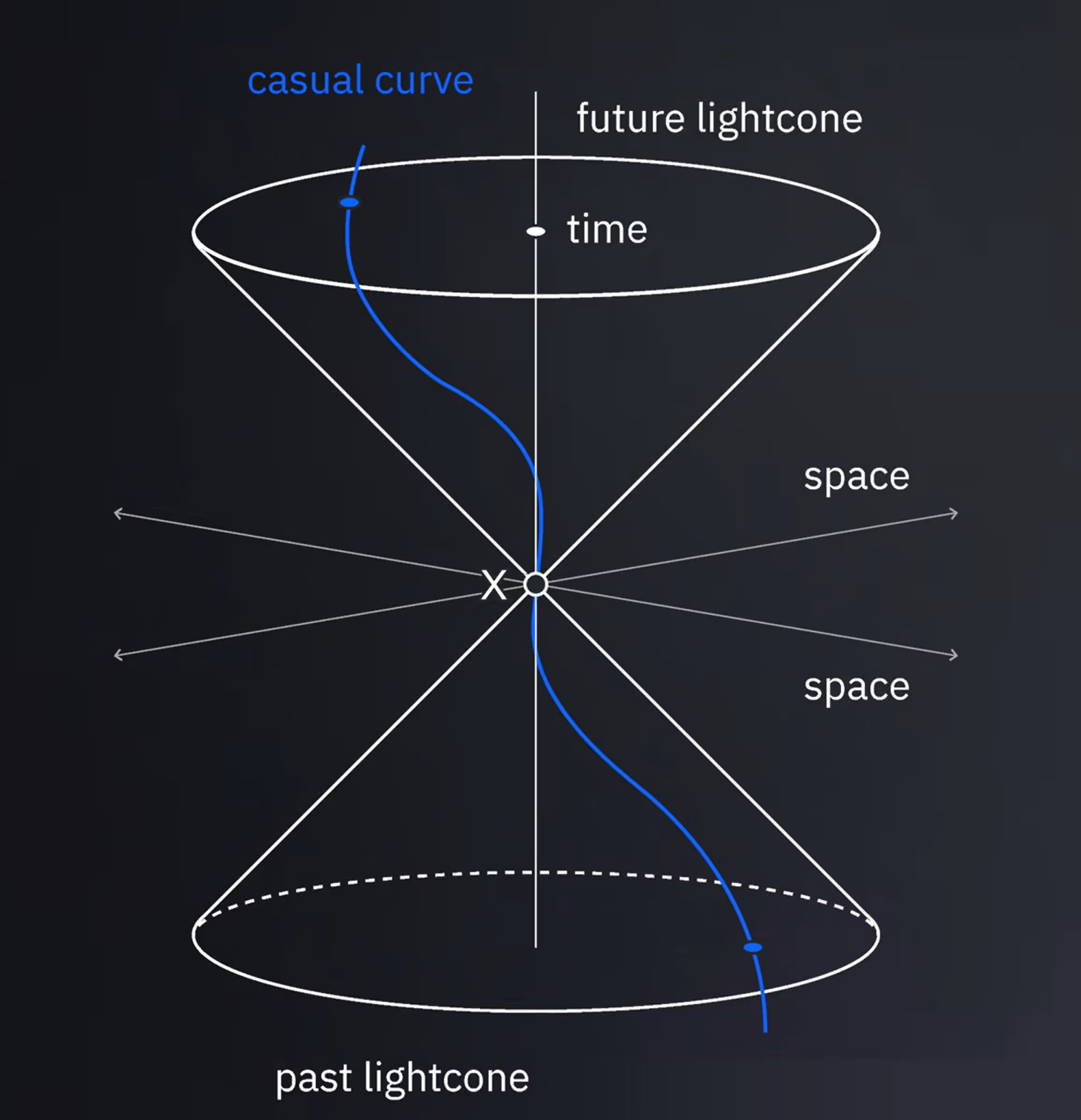
A similar concept applies in quantum circuits.

Consider a large circuit in which only a low-weight observable is of interest. A low-weight observable acts nontrivially on only a few qubits. Low-weight observables are of interest for many reasons. For example, they can represent the following:

• Individual terms within a larger Hamiltonian
• A localized interaction region
• Information collected onto a small set of ancilla qubits
• Other observables that involve only a few qubits

Not every error in the circuit can affect the measurement outcome. This is especially true of Pauli errors, or any error that can be modeled as a set of Pauli operations. For example, look at the following circuit:

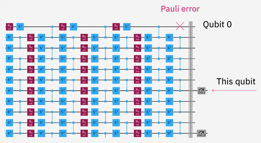
A Pauli error on qubit 0 in the final layer cannot influence the measurement on qubit 6, because there is no connecting gate that could propagate the error from qubit 0 to qubit 6. Note that this argument does not apply to certain non-unitary errors. For example, a T1-like transition to the ground state on qubit 0 collapses qubit 0 to a computational basis state. If qubits 0 and 6 were previously entangled (as they are in this circuit), the non-unitary error on qubit 0 can affect qubit 6. The following discussion focuses on errors that can be represented as Pauli operations, or as probabilistic mixtures of Pauli operations.

In the last layer, only a Pauli error on qubit 5 or qubit 6 can directly affect the measurement on qubit 6.

In the entangling layer before that one, qubits 5 and 6 are entangled with qubits 4 and 7, respectively. Therefore, in that entangling layer or just before it, a Pauli error on any of those four qubits can affect the later measurement. You can continue to trace backward through the circuit to find the subset of gates and qubits that are causally connected to the measurement. This causal set forms a cone-shaped region in space (qubits) and time (layers), which gives rise to the term lightcone. The exact shape of the region varies from circuit to circuit. Because this analysis depends on hardware connectivity and gate placement, it is most useful after transpilation, routing, and layout optimization.

Beyond causal connectivity

Shaded lightcones extend this idea by also considering which types of errors matter.

For example, note the following:

• A Z error immediately before a Z-basis measurement has no effect on the measurement outcome.
• An X error immediately before a Z-basis measurement can dramatically change the result.

Some error types therefore deserve more mitigation effort than others. This distinction can substantially reduce the overhead of techniques such as PEC. In practice, the addon generates separate sensitivity analyses for each of the following error types:

• X errors
• Z errors
• Y (or XZ up to a phase) errors

This error sensitivity generally looks different for each error type, because different causally connected errors have different impacts on the measurement. Note also that the sensitivity changes throughout the circuit. An X error immediately before measurement might be highly damaging, while an error that occurs many layers earlier might have a smaller effect after it propagates through a highly entangled state.

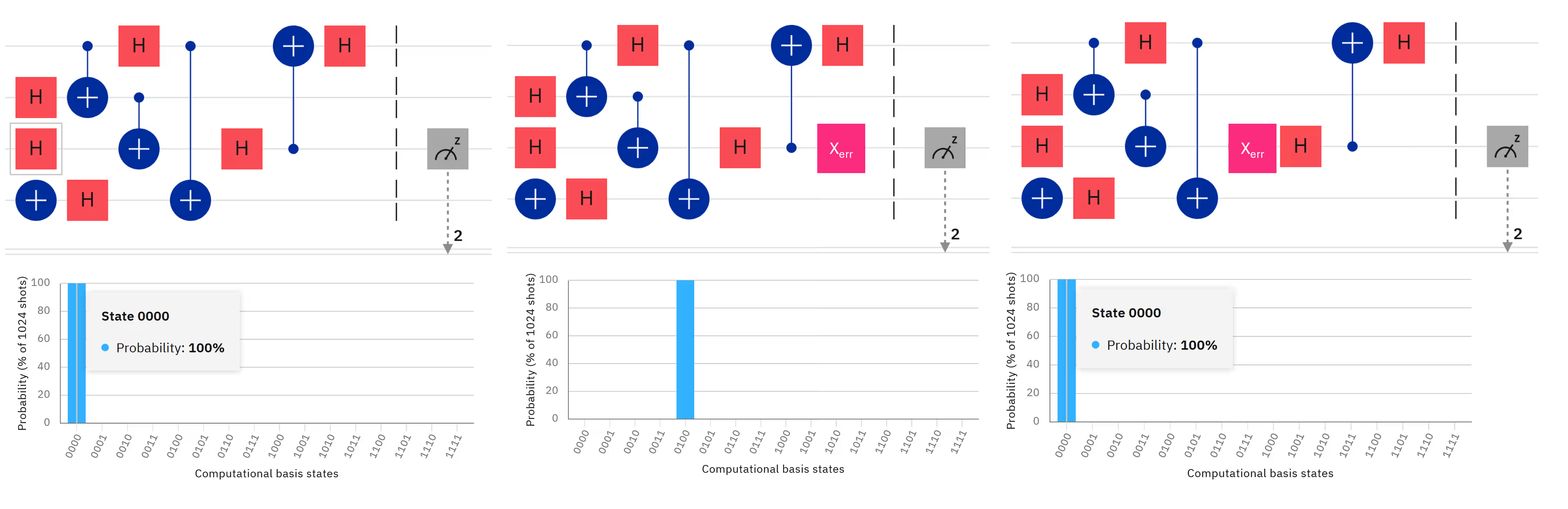
Shaded lightcones quantify this difference by assigning a sensitivity value to potential errors throughout the circuit.

The resulting maps indicate the following:

• Where errors matter
• Which error types matter
• How strongly they influence the final observable

Shaded lightcones do not mitigate errors themselves, but they can help focus mitigation effort where it provides the greatest benefit.

Learn and inject noise

After a circuit has been constructed, optimized, and annotated, two complementary tasks remain: learning the noise, and using the noise model (for example, to inject noise or to propagate the effects of noise).

NoiseLearnerV3

NoiseLearnerV3 is the current tool for noise learning. The previous NoiseLearner interface accepted entire circuits and produced Pauli-Lindblad noise models. NoiseLearnerV3 instead operates directly on boxed circuit instructions. In summary, NoiseLearnerV3 does the following:

• Accepts collections of labeled circuit layers
• Reuses information from repeated layers
• Supports measurement-noise learning
• Supports post-processing of learned models
• Enables noise injection and scaling workflows

This design aligns closely with the layer-oriented workflow of Samplomatic. In particular, NoiseLearnerV3 uses the following methods for each instruction set:

• Pauli-Lindblad learning for gate operations
• TREX-based learning for measurements

You can then use a learned noise model in many of the methods that we have already covered. For example, recall that zero-noise extrapolation (ZNE) with gate folding can lead to intractably deep circuits. The alternative method for scaling noise in that case was to sample from a known noise model, which effectively increases the noise level, even by non-integer factors. This method, probabilistic error amplification (PEA), is a good example of how you can use a noise model to mitigate errors. A good noise model is also required for probabilistic error cancellation (PEC) and propagated noise absorption (PNA).

In short, with a high-quality noise model, noise becomes a programmable resource rather than only a source of error.

Shaded lightcones versus NoiseLearnerV3

NoiseLearnerV3 and SLC are closely related, but they take distinct inputs and answer different questions. SLC determines where to focus mitigation effort. NoiseLearnerV3 characterizes the actual noise present in those regions. These processes also involve different kinds of overhead. The following table summarizes these differences.

	Shaded lightcones	NoiseLearnerV3
Purpose	Identifies where mitigation matters	Learns how errors behave
Overhead	Primarily classical overhead	Requires hardware executions
Output	Produces sensitivity maps	Produces noise-channel descriptions
Input	Uses circuit structure and operator propagation	Uses circuit structure and experimental hardware data

Executor and runtime execution

Executor performs the final execution step. It can operate on either of the following inputs:

• A template circuit and samplex generated by Samplomatic
• A conventional quantum circuit without Samplomatic

With this flexibility, you can adopt as many or as few components of the directed execution workflow as you need.

Executor works closely with Samplomatic, which manages randomization choices, shot allocation, noise-injection selections, and related execution metadata, as described previously.

For practical examples of the directed execution model, see the Directed execution model guide as well as the tutorials and Qiskit addon documentation on IBM Quantum® Platform.

Conclusion

Modern quantum workflows increasingly rely on a collection of complementary tools rather than a single execution primitive.

These tools support every stage of the workflow:

• Problem mapping
• Circuit construction
• Transpilation and optimization
• Error suppression
• Error mitigation
• Noise learning
• Structured execution
• Post-processing

Together, tools such as Samplomatic, Executor, NoiseLearnerV3, shaded lightcones, propagated noise absorption, circuit cutting, and AQC-Tensor provide significantly more control than earlier execution models.

The field continues to evolve rapidly. As quantum processors become larger and more connected, these techniques are likely to play an increasingly important role in achieving useful quantum advantage, and eventually in integrating seamlessly with fault-tolerant quantum computing workflows.