Error suppression and tailoring

Error suppression can refer to any technique that anticipates and tries to avoid certain types of noise and errors. This is easiest to explain through concrete examples, but keep in mind that these methods are not limited to the examples shown here, and new methods are continually being explored. Sometimes it is not possible to suppress errors, but it is possible to affect how they accumulate. If we can make errors accumulate more slowly, we might describe this as suppressing the overall error, but it is more accurately viewed as noise tailoring. In this lesson we cover canonical examples of error suppression (dynamical decoupling) and of noise tailoring/shaping (Pauli twirling).

A video to accompany this lesson will launch in the next few days, and will be embedded here.

Dynamical decoupling

Let us begin with a very simple state on a single qubit, and introduce a simple noise model. This is insufficient to completely explain dynamical decoupling, but it gives us a clear example. Suppose we have a qubit prepared in a superposition state using a Hadamard gate:

$$|\psi\rangle = H|0\rangle = \frac{1}{\sqrt{2}}\left( |0\rangle +|1\rangle \right).$$

This state is visualized on the Bloch sphere as shown below on the left. In the ideal case with zero noise, this qubit would remain in this state until the next operation is carried out. However, we know from the previous lesson that this is not what we observe. Noise causes the quantum information to degrade.

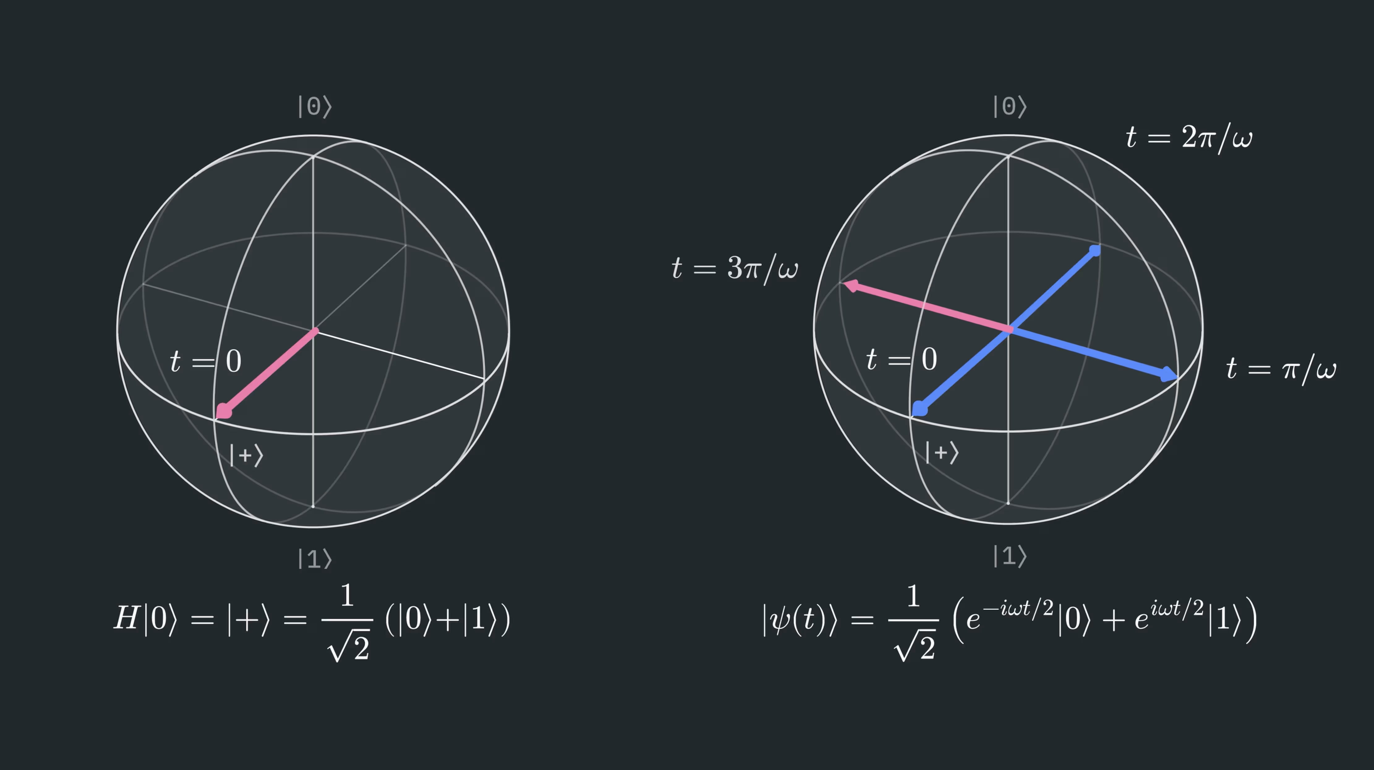
Noise or environmental coupling can cause the relative phase between the basis states to change. That is, the probabilities of $|0\rangle$ and $|1\rangle$ do not change, as the absolute values of their coefficients do not change. Rather, the phases of the amplitudes change, altering their real and imaginary components. To make this discussion more concrete, let us consider one type of interaction that can cause this: coupling to a magnetic field oriented in the Z direction: $\vec{B} = (0,0,B_0)$.

Consider what happens to the state $|+\rangle$ as time passes:

$$|\psi(t)\rangle = e^{-iHt/\hbar}|\psi(0)\rangle \rightarrow e^{-iZ\omega_B t/2}|\psi(0)\rangle$$

Here we have used the fact that a magnetic field in the Z direction causes precession about the Z axis with a frequency $\omega_B$ that depends on the effective magnetic moment and magnetic field strength. The details are less important than the fact that this interaction causes evolution about the Z axis, resulting in opposite phase accumulation for the two computational basis states. Applying this operator to each term in $|\psi\rangle$, we find the following:

$$|\psi(t)\rangle = e^{-iZ\omega_B t/2}\frac{1}{\sqrt{2}}\left( |0\rangle +|1\rangle \right) =\frac{1}{\sqrt{2}}\left( e^{-i\omega_B t/2}|0\rangle +e^{i\omega_B t/2}|1\rangle \right)$$

This time-dependent phase corresponds to precession about the Z axis in the Bloch sphere picture. This is shown in the right half of the figure above.

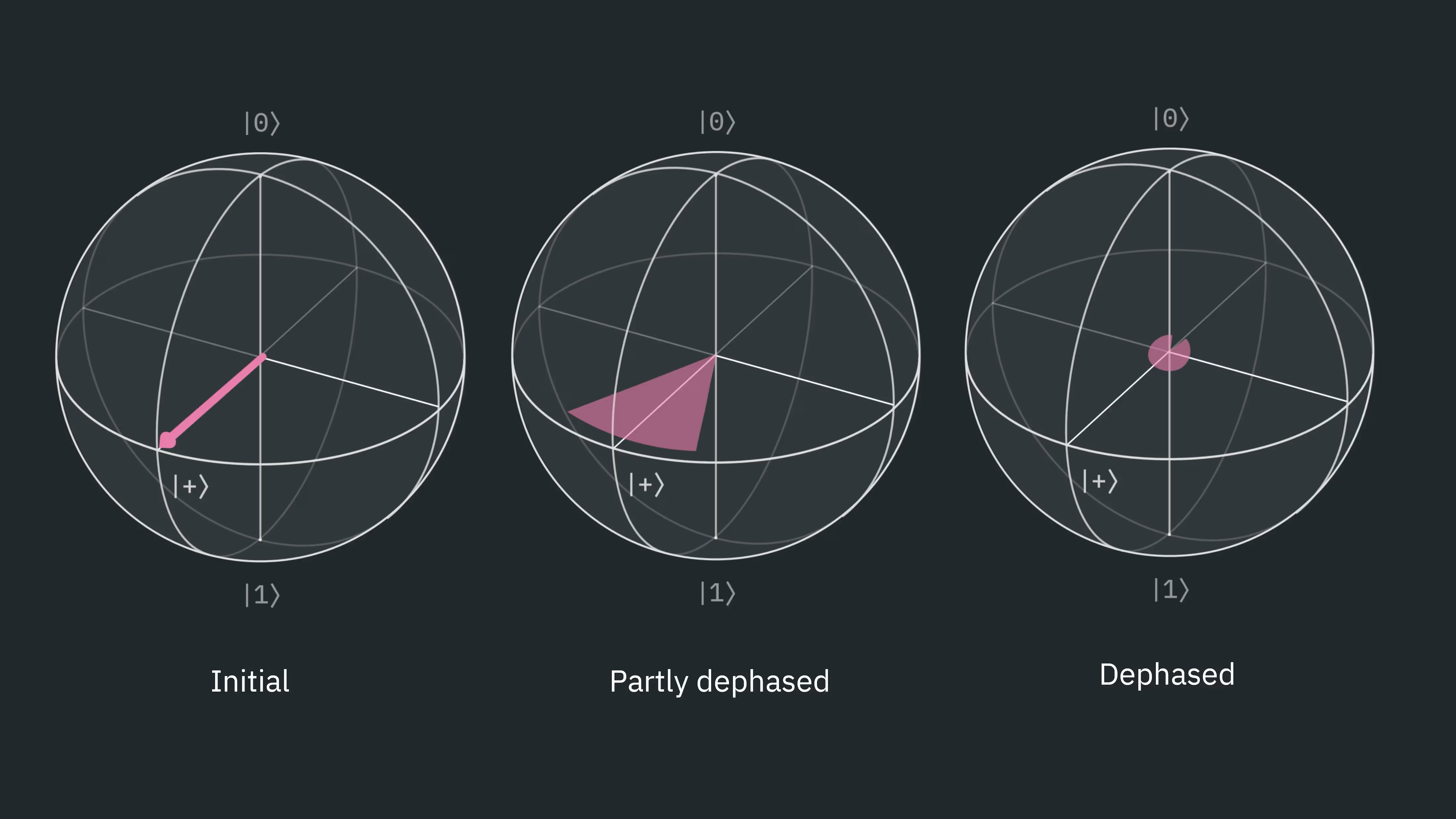
If we knew that this interaction were occurring in a controlled way, we could predict it. To model this type of noise, we instead consider a distribution of possible magnetic field strengths, each occurring with some classical probability (other sources of noise would need to be modeled differently). We need to consider what happens when there is a non-zero classical probability that the state has not rotated at all, and also some probability that it has rotated by a small amount, or even by a large amount. This distribution of possible rotations is the reason for the spreading of the state in the Bloch sphere picture below. If there is more such dephasing noise, the phase will be less well-defined. In the limit of strong dephasing, the qubit becomes completely dephased, corresponding to the loss of the quantum coherence stored in the state.

Of course, in an experiment we have no idea what random coupling will occur. What can we do about this?

Suppose that the environmental coupling remains approximately constant over a time interval $2t_0$. Consider what would happen if we followed this prescription:

• Allow the phase to change for time $t_0$
• Apply an X gate to the qubit
• Allow the same environmental coupling to occur for a further time $t_0$
• Apply a second X gate

After the initial time evolution, we would have exactly the state above. Applying the first X gate we have:

$$X|\psi(t_0)\rangle = \frac{1}{\sqrt{2}}\left( e^{-i\omega_B t_0/2}|1\rangle +e^{i\omega_B t_0/2}|0\rangle \right)$$

Now when the second interval of $t_0$ passes, the same interaction takes place. But now the amplitudes are associated with the opposite Z eigenstates, meaning the sign of the rotation about the Z axis has switched. After allowing the system to evolve in time for another $t_0$ we have the state:

$$e^{-iZ\omega_B (t-t_0)/2}\frac{1}{\sqrt{2}}\left( e^{-i\omega_B t_0/2}|1\rangle +e^{i\omega_B t_0/2}|0\rangle \right) =\frac{1}{\sqrt{2}}\left( e^{-i\omega_B (t-t_0)/2}e^{i\omega_B t_0/2}|1\rangle +e^{i\omega_B (t-t_0)/2}e^{-i\omega_B t_0/2}|0\rangle \right)$$

And inserting $t = 2t_0$ we have:

$$|\psi(2t_0)\rangle=\frac{1}{\sqrt{2}}\left(|1\rangle +|0\rangle \right)$$

Applying the final X gate does nothing in this case, but it is generally necessary:

$$|\psi(2t_0)\rangle = \frac{1}{\sqrt{2}}\left(|0\rangle +|1\rangle \right) = |\psi(t=0)\rangle$$

We have recovered the original quantum state, including its relative phase. This process is an especially simple example of dynamical decoupling.

More generally, dynamical decoupling (DD) involves inserting some single-qubit gates to reduce the effect of interactions with systems outside the qubit (decoupling it from the environment). The complete refocusing of all possible phase histories back to the original state, as shown above, is somewhat idealized, but it is still a possible scenario. Let's discuss when DD is useful and what caveats exist.

Check your understanding

In the text above, we stepped through the effect of an XX DD sequence on the initial state $|+\rangle$. Check whether the same steps above also return the state $|+i\rangle$ back to its initial state under the same assumptions of a slowly-varying magnetic field along the z direction.

Answer

$$|\psi(t)\rangle = e^{-iZ\omega_B t/2}\frac{1}{\sqrt{2}}\left( |0\rangle +i|1\rangle \right) =\frac{1}{\sqrt{2}}\left( e^{-i\omega_B t/2}|0\rangle +i e^{i\omega_B t/2}|1\rangle \right)$$

After the initial time evolution, we would have exactly the state above. Applying the first X gate we have:

$$X|\psi(t_0)\rangle = \frac{1}{\sqrt{2}}\left( e^{-i\omega_B t_0/2}|1\rangle +i e^{i\omega_B t_0/2}|0\rangle \right)$$

Now when the second interval of $t_0$ passes, the same interaction takes place. But now the amplitudes are associated with the opposite Z eigenstates, meaning the sign of the rotation about the Z axis has switched. After allowing the system to evolve in time for another $t_0$ we have the state:

$$e^{-iZ\omega_B (t-t_0)/2}\frac{1}{\sqrt{2}}\left( e^{-i\omega_B t_0/2}|1\rangle +i e^{i\omega_B t_0/2}|0\rangle \right) =\frac{1}{\sqrt{2}}\left( e^{-i\omega_B (t-t_0)/2}e^{i\omega_B t_0/2}|1\rangle +i e^{i\omega_B (t-t_0)/2}e^{-i\omega_B t_0/2}|0\rangle \right)$$

And inserting $t = 2t_0$ we have

$$|\psi(2t_0)\rangle=\frac{1}{\sqrt{2}}\left(|1\rangle +i |0\rangle \right)$$

Applying the final X gate, we have:

$$|\psi(2t_0)\rangle = \frac{1}{\sqrt{2}}\left(|0\rangle +i |1\rangle \right) = |\psi(t=0)\rangle = |+i\rangle$$

When to use DD

The first and most obvious caveat is that we assumed a purely dephasing channel in our treatment. Real-world interactions typically produce a mixture of dephasing and other error mechanisms. In the treatment above, we chose to apply X gates specifically. This is referred to as an XX sequence in dynamical decoupling. This particular sequence is appropriate for purely dephasing errors. But there are other sequences that might be more broadly applicable, like XY4 (shown in the circuit diagram below) and the more complex XY8.

Another caveat is that dynamical decoupling adds single-qubit gates, which can add single-qubit errors due to gate imperfections or even crosstalk. These single-qubit error rates are typically much lower than multi-qubit gate errors, so this is usually not a major concern, but it is something to keep in mind if many qubits are employing DD many times throughout your circuit.

DD is useful when the external coupling has time to affect the state of the qubit. Because qubits are painstakingly well isolated and external couplings should be weak, this type of noise is most noticeable when a qubit sits idle for long periods. For short idle times, the effect of DD could be to add single-qubit gate errors while suppressing very little noise; the fidelity of your circuit could actually be reduced.

Key takeaway: Use dynamical decoupling when qubits remain idle for sufficiently long periods, and pay attention to the type of DD sequence being used.

Dynamical decoupling using Qiskit

Let us explore the use of DD by examining the case of several qubits prepared in the $|+\rangle$ state, which then remain idle for a long time. In the absence of errors, preparing the multi-qubit state $|\psi\rangle = |+\rangle^{\otimes N}$ and then applying a Hadamard gate before measurement (thereby measuring in the X basis) should always yield 0. With noise, the measurement outcome will be 0 only a fraction of the time rather than with 100% probability. We calculate the average X expectation value across multiple qubits. That is, we are interested in the following:

$$f\equiv \frac{1}{N}\sum_{j=0}^{N-1}{\langle\Psi | X_j |\Psi\rangle}$$

where $X_j \equiv III..X...II$ with the X operator in the $j^{th}$ position from the right and $|\Psi\rangle$ is the state of the entire system.

This circuit contains intentional delays, which is somewhat contrived for a benchmark. However, it is very common for real circuits to contain qubits that sit idle during part of the execution. You can think of this as a simplified model of a more complex circuit in which some qubits remain idle for part of the computation. This type of benchmarking based on the evolution of $|+\rangle$ states is often referred to as Ramsey benchmarking.

We begin by loading the necessary packages and configuring the service.

# Added by doQumentation — required packages for this notebook
!pip install -q matplotlib numpy qiskit qiskit-aer qiskit-ibm-runtime

# Load key packages

from qiskit_ibm_runtime import QiskitRuntimeService
from qiskit_ibm_runtime import SamplerV2 as Sampler
from qiskit.transpiler.preset_passmanagers import generate_preset_pass_manager
from qiskit import QuantumRegister, ClassicalRegister, QuantumCircuit
import numpy as np

# --------- Configuration ----------

service = QiskitRuntimeService()  # assumes credentials are saved
backend = service.backend("ibm_fez")  # adjust if needed

Now we define some helper functions. First, we want to address the point about long idle times. What exactly does "long" mean in this context? We could simply report the idle time in microseconds. However, it is useful to know how many two-qubit gates could be executed during that same interval. This makes the idle times more directly indicative of the circuit depth that could have been executed during the same period. The first helper function gets the two-qubit gate native to the backend and determines the duration of that gate.

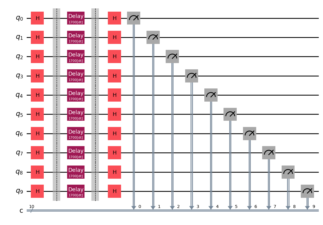
The second function simply creates a Ramsey circuit (one with qubits in the $|+\rangle$ state), implements a delay, rotates using an H gate, and then measures. Recall that a Hadamard gate (H) maps $|+\rangle$ to $|0\rangle$, so measuring $|0\rangle$ in the Z basis after the Hadamard corresponds to the qubit having been in $|+\rangle$ immediately before the Hadamard.

Our final function converts the raw counts of 0 and 1 measurement outcomes into an expectation value of X.

from typing import Tuple
from qiskit.providers import Backend
from numpy.typing import NDArray

# --------- Utilities ----------
def detect_twoq_gate_and_duration(
    backend: Backend, pair: tuple[int, int] = (0, 1)
) -> Tuple[str, float]:
    props = backend.properties()
    candidates = ["cx", "ecr", "cz"]
    for name in candidates:
        try:
            dur = props.gate_length(name, list(pair))
            if dur is not None:
                return name, dur
        except Exception:
            pass
    raise RuntimeError(
        "Could not find a two-qubit gate duration among cx/ecr/cz on this backend."
    )

def make_multiqubit_ramsey_circuit(n: int, delay_dt_ticks: int) -> QuantumCircuit:
    q = QuantumRegister(n, "q")
    c = ClassicalRegister(n, "c")
    qc = QuantumCircuit(q, c)

    qc.h(q)
    qc.barrier()

    for i in range(n):
        qc.delay(delay_dt_ticks, q[i], unit="dt")
    qc.barrier()

    qc.h(q)
    qc.measure(q, c)
    return qc

def counts_to_x_expectations(counts: dict[str, int], n: int) -> NDArray[np.float64]:
    total = sum(counts.values())
    if total == 0:
        return np.zeros(n)

    p0 = np.zeros(n, dtype=float)
    for bitstring, cnt in counts.items():
        bits_rev = bitstring[::-1]
        for i in range(n):
            if bits_rev[i] == "0":
                p0[i] += cnt
    p0 /= total
    return 2.0 * p0 - 1.0

Now we specify the details of our test, including the number of qubits and the gate sequence to be used in DD (in this case XX). Note especially that we set the optimization level to zero. In practice, you would often select a higher optimization level; here we use level 0 to ensure that the effects of the errors targeted by DD remain visible. Finally, we determine the characteristic time for two-qubit gates on this backend and print some relevant times.

n_qubits = 10  # number of qubits to test in parallel
shots = 4096
opt_level = 0  # we want to ignore optimization for now
num_steps = 6  # number of delay points
gates_per_step = 20  # "equivalent 2q gates" per step
dd_sequence = "XX"  # "XX" for your request; you might try "XY4" too

# --------- Derive timing: dt and 2q gate time ----------
dt = backend.dt  # seconds per dt
twoq_name, t2q = detect_twoq_gate_and_duration(backend, (0, 1))  # seconds
delay_unit_dt = int(round(t2q / dt))  # dt ticks equivalent to one 2q gate

print(f"Backend: {backend.name}")
print(f"dt = {dt*1e9:.3f} ns per tick")
print(f"Using 2q gate '{twoq_name}' with duration ~ {t2q*1e9:.1f} ns")
print(f"One 2q gate ≈ {delay_unit_dt} dt ticks")

Backend: ibm_fez
dt = 4.000 ns per tick
Using 2q gate 'cz' with duration ~ 68.0 ns
One 2q gate ≈ 17 dt ticks

We now construct our circuits and transpile them for our chosen backend.

# --------- Build circuits for a sweep of delays ----------
pm = generate_preset_pass_manager(optimization_level=opt_level, backend=backend)

equiv_gates_list = [
    j * gates_per_step for j in range(num_steps)
]  # e.g., 0, 100, 200, ...
delay_dt_list = [int(round(delay_unit_dt * m)) for m in equiv_gates_list]
delay_us_list = [(dt * d) * 1e6 for d in delay_dt_list]  # for printing/plotting

circuits = []
for delay_dt in delay_dt_list:
    qc = make_multiqubit_ramsey_circuit(n_qubits, delay_dt)
    qc_isa = pm.run(qc)  # ISA-level scheduling/placement; DD is handled at runtime
    circuits.append(qc_isa)

print("Delay sweep (approx microseconds):", [f"{t:.2f}" for t in delay_us_list])

Delay sweep (approx microseconds): ['0.00', '1.36', '2.72', '4.08', '5.44', '6.80']

We should visualize at least one circuit to ensure we have coded our circuit with the desired states and delays. It might be easier to visualize the pre-transpiled circuit qc, or you might check the transpiled one qc_isa.

qc.draw("mpl")

Execute

We're finally ready to execute on hardware. We use Sampler to obtain many measurements of each qubit, and we will use it twice: once with DD explicitly turned off, and once with DD turned on and using the XX gate sequence.

# --------- Run: NO DD ----------
sampler = Sampler(mode=backend)
sampler.options.default_shots = shots
sampler.options.dynamical_decoupling.enable = False

job = sampler.run(circuits)
res_nodd = job.result()
job_id = job.job_id()  # job id for dd off/false
print("job number for no dd is ", job_id)

# --------- Run: WITH DD (XX) ----------
sampler = Sampler(mode=backend)
sampler.options.default_shots = shots
sampler.options.dynamical_decoupling.enable = True
sampler.options.dynamical_decoupling.sequence_type = (
    dd_sequence  # "XX" first; you can try "XY4" too
)
sampler.options.dynamical_decoupling.scheduling_method = "alap"
sampler.options.dynamical_decoupling.extra_slack_distribution = "middle"

job = sampler.run(circuits)
res_dd = job.result()
job_id = job.job_id()  # job id for dd on/XX
print("job number for dd using XX is ", job_id)

We can extract the counts from the various circuits.

# --------- Extract counts per circuit ----------

from typing import Iterable, Any

def extract_counts_list(res: Iterable[Any]) -> list[dict[str, int]]:
    counts_list: list[dict[str, int]] = []

    for r in res:  # each r corresponds to one circuit
        counts: dict[str, int] = r.data.c.get_counts()
        counts_list.append(counts)

    return counts_list

counts_list_nodd = extract_counts_list(res_nodd)
counts_list_dd = extract_counts_list(res_dd)

Post-processing

We now have the counts from the measurement, but we want to turn that into the expectation value of X and then average those expectation values across all the qubits we used, to learn about the preservation of phase information. For that we use our counts_to_x_expectations function defined earlier.

# --------- Compute X-expectations and a scalar contrast ----------
# For each circuit (each delay), compute per-qubit <X> and average absolute contrast.

xexp_nodd = []
xexp_dd = []
contrast_nodd = []
contrast_dd = []

for counts in counts_list_nodd:
    x_vec = counts_to_x_expectations(counts, n_qubits)
    xexp_nodd.append(x_vec)
    contrast_nodd.append(float(np.mean(np.abs(x_vec))))  # average |<X>| across qubits

for counts in counts_list_dd:
    x_vec = counts_to_x_expectations(counts, n_qubits)
    xexp_dd.append(x_vec)
    contrast_dd.append(float(np.mean(np.abs(x_vec))))

# --------- Print a small summary ----------
print("\n=== Summary (average |<X>| per delay) ===")
for m, d_us, c0, c1 in zip(equiv_gates_list, delay_us_list, contrast_nodd, contrast_dd):
    print(
        f"Delay ~ {m:4d} * {twoq_name}  (~{d_us:7.2f} µs):  NoDD={c0: .3f},  DD({dd_sequence})={c1: .3f}"
    )

# Optionally, inspect per-qubit values for the last delay point
print("\nPer-qubit <X> (abs) at the longest delay:")
print("NoDD:", np.round(np.abs(xexp_nodd[-1]), 3))
print("DD  :", np.round(np.abs(xexp_dd[-1]), 3))

=== Summary (average |<X>| per delay) ===
Delay ~    0 * cz  (~   0.00 µs):  NoDD= 0.954,  DD(XX)= 0.961
Delay ~   20 * cz  (~   1.36 µs):  NoDD= 0.827,  DD(XX)= 0.927
Delay ~   40 * cz  (~   2.72 µs):  NoDD= 0.793,  DD(XX)= 0.900
Delay ~   60 * cz  (~   4.08 µs):  NoDD= 0.729,  DD(XX)= 0.876
Delay ~   80 * cz  (~   5.44 µs):  NoDD= 0.661,  DD(XX)= 0.854
Delay ~  100 * cz  (~   6.80 µs):  NoDD= 0.586,  DD(XX)= 0.826

Per-qubit <X> (abs) at the longest delay:
NoDD: [0.05  0.744 0.712 0.867 0.844 0.234 0.473 0.755 0.59  0.587]
DD  : [0.583 0.89  0.921 0.88  0.908 0.832 0.893 0.773 0.807 0.773]

Finally, let's plot our results.

import matplotlib.pyplot as plt

fig, ax = plt.subplots()

# Add values with no DD
ax.scatter(
    equiv_gates_list, contrast_nodd, c="blue", linestyle="-", label="No DD", alpha=0.7
)

## Add values with DD
ax.scatter(
    equiv_gates_list, contrast_dd, c="red", linestyle="-", label="With DD", alpha=0.7
)

# Add labels and plot
ax.set_xlabel("Idle Time in # of 2-qubit gates")
ax.set_ylabel("<X>")
ax.legend()
ax.set_title("Dephasing and DD")
ax.grid(True)

plt.show()

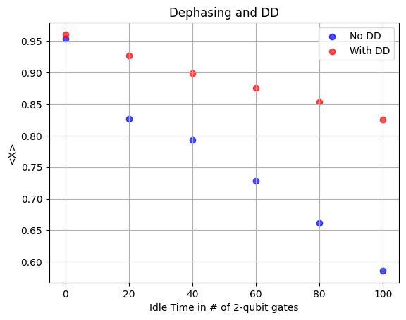
As you can see, with no explicit delay the expectation values are indeed near 1, which we would expect if all phase information were preserved. If all phase information were lost, there would be no preference for the final rotation to produce $|0\rangle$ rather than $|1\rangle$, and the average expectation value would approach zero. In the data, we see that as delay times increase, the average expectation value of X decreases, starting to approach zero. Note that DD has been very effective here; the expectation values with DD are typically more than 20% better (closer to 1) than the values without DD. But also note that the first delayed data point corresponds to a delay roughly equivalent to 100 two-qubit gate operations. This reinforces the point that DD is most useful when qubits remain idle for relatively long periods.

Check your understanding

If we apply DD using XY4 to the same circuit as before, do you expect it to yield results that are much better, much worse, or about the same, as DD using XX? Explain.

Answer

About the same, perhaps slightly worse. The circuit we used had states rotated into the XY plane. This state stores information primarily in its phase, making it especially sensitive to dephasing errors rather than T1 relaxation. XY4 might help with a wider variety of errors, but XX is already optimized to help the circuit we are using. XY4 might be just as good, but would not add anything substantial, or the fact that XY4 contains more gates might allow additional gate errors to make the results slightly worse.

The last result used the simplest DD gate sequence XX. Let's see how to implement a more complex sequence, XY4. We define a Sampler in the next section.

# --------- Run: WITH DD (XY4) ----------
dd_sequence = "XY4"

sampler = Sampler(mode=backend)
sampler.options.default_shots = shots
sampler.options.dynamical_decoupling.enable = True
sampler.options.dynamical_decoupling.sequence_type = dd_sequence
sampler.options.dynamical_decoupling.scheduling_method = "alap"
sampler.options.dynamical_decoupling.extra_slack_distribution = "middle"

job = sampler.run(circuits)
res_xy4 = job.result()
job_id = job.job_id()  # job id for dd on/XY4
print("job number for dd using Xy4 is ", job_id)

job number for dd using Xy4 is  d6k6ti860irc7395d3hg

# --------- Extract counts per circuit ----------

counts_list_xy4 = extract_counts_list(res_xy4)
# --------- Compute X-expectations and a scalar contrast ----------
# For each circuit (each delay), compute per-qubit <X> and average absolute contrast.
xexp_xy4 = []
contrast_xy4 = []

for counts in counts_list_xy4:
    x_vec = counts_to_x_expectations(counts, n_qubits)
    xexp_xy4.append(x_vec)
    contrast_xy4.append(float(np.mean(np.abs(x_vec))))  # average |<X>| across qubits

# --------- Print a small summary ----------
print("\n=== Summary (average |<X>| per delay) ===")
for m, d_us, c0, c1, c2 in zip(
    equiv_gates_list, delay_us_list, contrast_nodd, contrast_dd, contrast_xy4
):
    print(
        f"Delay ~ {m:4d} * {twoq_name}  (~{d_us:7.2f} µs):  NoDD={c0: .3f},  DD({dd_sequence})={c1: .3f}"
    )

# Optionally, inspect per-qubit values for the last delay point
print("\nPer-qubit <X> (abs) at the longest delay:")
print("NoDD:", np.round(np.abs(xexp_nodd[-1]), 3))
print("DD XX :", np.round(np.abs(xexp_dd[-1]), 3))
print("DD XY4 :", np.round(np.abs(xexp_xy4[-1]), 3))

=== Summary (average |<X>| per delay) ===
Delay ~    0 * cz  (~   0.00 µs):  NoDD= 0.968,  DD(XY4)= 0.968
Delay ~  100 * cz  (~   6.80 µs):  NoDD= 0.612,  DD(XY4)= 0.839
Delay ~  200 * cz  (~  13.60 µs):  NoDD= 0.462,  DD(XY4)= 0.705
Delay ~  300 * cz  (~  20.40 µs):  NoDD= 0.339,  DD(XY4)= 0.580
Delay ~  400 * cz  (~  27.20 µs):  NoDD= 0.225,  DD(XY4)= 0.481
Delay ~  500 * cz  (~  34.00 µs):  NoDD= 0.204,  DD(XY4)= 0.393

Per-qubit <X> (abs) at the longest delay:
NoDD: [0.002 0.208 0.447 0.034 0.286 0.306 0.322 0.044 0.163 0.232]
DD XX : [0.433 0.669 0.526 0.516 0.572 0.284 0.303 0.055 0.365 0.208]
DD XY4 : [0.38  0.662 0.521 0.538 0.621 0.252 0.353 0.038 0.239 0.073]

import matplotlib.pyplot as plt

fig, ax = plt.subplots()

# Add values with no DD
ax.scatter(
    equiv_gates_list, contrast_nodd, c="blue", linestyle="-", label="No DD", alpha=0.7
)

## Add values with DD using XX sequence
ax.scatter(
    equiv_gates_list, contrast_dd, c="red", linestyle="-", label="With XX", alpha=0.7
)

## Add values with DD using XY4 sequence
ax.scatter(
    equiv_gates_list,
    contrast_xy4,
    c="black",
    linestyle="-",
    label="With XY4",
    alpha=0.7,
)

# Add labels and plot
ax.set_xlabel("Idle Time in # of 2-qubit gates")
ax.set_ylabel("<X>_av")
ax.legend()
ax.set_title("Dephasing and DD")
ax.grid(True)

plt.show()

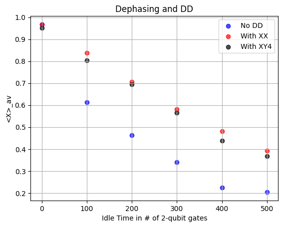
Here we see that XY4 is not appreciably different from XX. It might be very slightly worse due to additional gates in the XY4 sequence, but more importantly, we already explained why XX would have the desired effect in preserving phase specifically for a state like $|+\rangle$. There is no reason to think that for such an initial state, a different sequence would improve results.

Check your understanding

Verify that the XY4 sequence leaves the state unchanged up to a global phase.

Answer

$$\begin{aligned} YXYX|+\rangle & = YXYX(|0\rangle+|1\rangle)\\ & = YXY(|0\rangle+|1\rangle)\\ & = YX(i|1\rangle-i|0\rangle)\\ & = Y(i|0\rangle-i|1\rangle)\\ & = (-|0\rangle-|1\rangle)\\ & =-|+\rangle \end{aligned}$$

Pauli twirling

We should begin by noting that Pauli twirling is often used not as an error-suppression technique, but as an error-shaping technique: it makes noise/errors behave differently, sometimes more predictably, to enable other methods. Although Pauli twirling does not prevent errors, it might prevent their coherent accumulation.

In a quantum circuit, multiple different sources of error add together. The errors can add in different ways, notably coherently and incoherently. Coherent accumulation of errors means that noise or imperfect implementations all tend to drive errors in the same direction across multiple layers and gates. An example would be coherent over-rotation when applying a rotation gate.

Consider an ideal rotation gate, such as $R_x(\theta_0)$, which rotates about the X axis by exactly $\theta_0$. Of course, gate implementation is not perfect, and the actual rotation might be $\theta_0+\Delta\theta$ for one implementation, and it could even be the case that $\Delta\theta$ is always the same sign, and possibly similar in magnitude across many applications of $R_x(\theta)$. Thus repeated application of rotation gates can result in coherent accumulation of these many over-rotations (or under-rotations), $\Delta \theta$.

Incoherent error accumulation is just the opposite: errors in random directions with random signs, such that errors in different layers do not always interfere additively, but sometimes cancel or add in quadrature. Clearly incoherent errors accumulate more slowly in terms of the overall effect on the state of the qubit. A toy diagram of this is shown in the figure below. This is a simplification. Real quantum errors are not restricted to a two-dimensional Cartesian space; not all error contributions will have the same magnitude, and there are more complexities. But the intuition of a picture like this is useful: coherent errors tend to accumulate faster than incoherent ones.

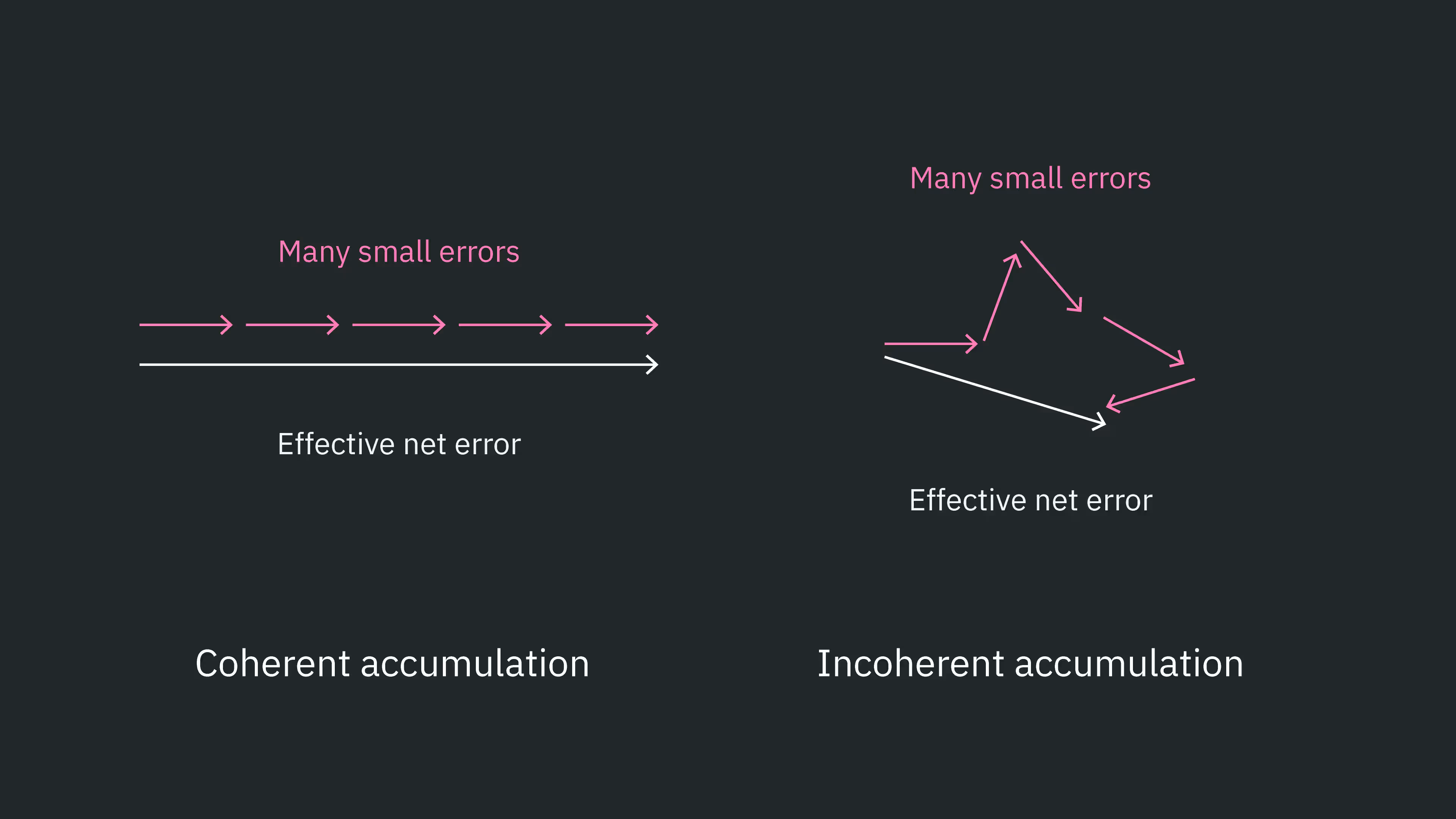
One can often obtain higher-fidelity results by turning coherent error accumulation into incoherent error accumulation. A primary way of accomplishing this is called Pauli twirling.

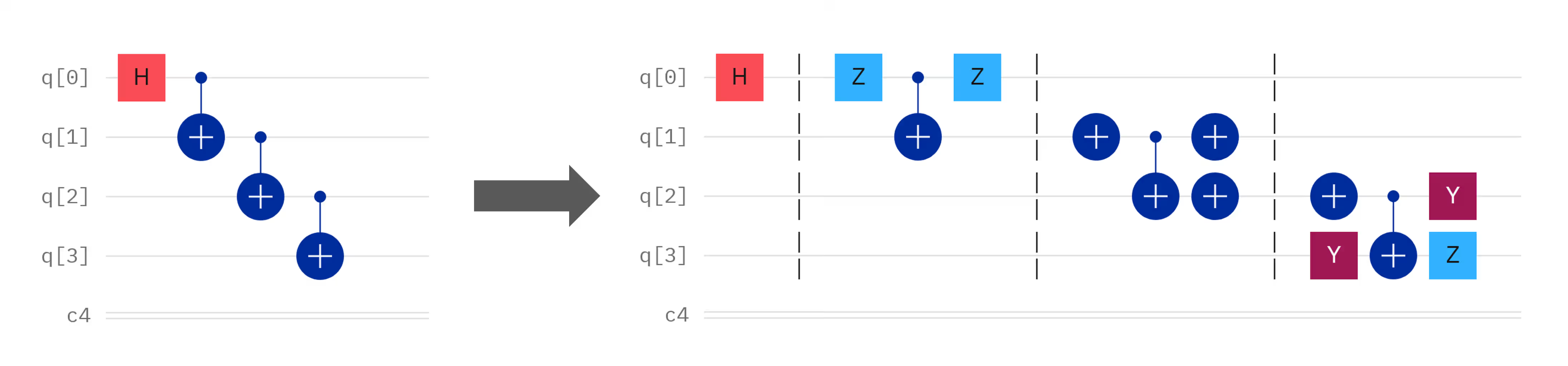
Pauli twirling refers to adding combinations of Pauli gates $P \in \{X, Y, Z, I\}$ before and after a desired gate operation $U$ in such a way that $P_1 U P_2 = U$. Here, $P_1$ and $P_2$ are not single Paulis, but collections of Pauli operators often acting on multiple qubits. You might sometimes see it stated that the action of the extra Pauli gates is "equivalent to the identity". But this is imprecise and potentially confusing. The Pauli gates are separated by $U$ and the goal is to leave the logical action of all gates equal to $U$. Sometimes $U$ is called the "payload" to distinguish this intended operation from the gates added for suppression. Some examples of Pauli twirling around a CNOT gate are shown below.

Let's walk through just one example to verify that twirling leaves the logical effect of the payload unchanged. Without loss of generality, let the two-qubit states involving $q_0$ and $q_1$ be:

$$|\psi_\text{init}\rangle = a|00\rangle + b|01\rangle + c|10\rangle + d|11\rangle$$

As always, we are using the qubit ordering convention $|q_1,q_0\rangle$. Applying a CX gate with $q_1$ as the target yields

$$CX|\psi_\text{init}\rangle = |\psi_\text{final}\rangle = a|00\rangle + b|11\rangle + c|10\rangle + d|01\rangle$$

Now let us consider the third circuit shown, using X gates for Pauli twirling. We could simply multiply the matrices together and verify that they yield a CNOT matrix. Alternatively, we can track the operation on an arbitrary quantum state through the circuit, as we do below. The states at different points in the circuit have been labeled a-d.

$$|\psi_a\rangle = a|00\rangle + b|01\rangle + c|10\rangle + d|11\rangle\\ |\psi_b\rangle = a|01\rangle + b|00\rangle + c|11\rangle + d|10\rangle\\ |\psi_c\rangle = a|11\rangle + b|00\rangle + c|01\rangle + d|10\rangle\\ |\psi_d\rangle = a|00\rangle + b|11\rangle + c|10\rangle + d|01\rangle$$

This is exactly $|\psi_\text{final}\rangle$ that we obtained before with no twirling. Indeed, this twirled gate sequence leaves the logical action of the payload unchanged. However, if different valid twirling sequences are selected randomly from layer to layer, coherent error accumulation can be converted into effectively stochastic (incoherent) error accumulation. To be clear, one does not choose a single twirling pattern and use it throughout the circuit. Instead, different valid twirling sequences are selected for different layers. An example with many entangling layers might look like this.

Check your understanding

Verify that the Pauli twirling in the fourth panel in the figure above also leaves the logical effect of the CNOT unchanged.

Answer

We follow the example above and show that the action on any arbitrary two-qubit state is equivalent to a CNOT operation. We will refer to the labeled points in this diagram.

$$\begin{aligned} |\psi_a\rangle & = a|00\rangle + b|01\rangle + c|10\rangle + d|11\rangle\\ |\psi_b\rangle & = ai|11\rangle + bi|10\rangle - ci|01\rangle - di|00\rangle\\ |\psi_c\rangle & = ai|01\rangle + bi|10\rangle - ci|11\rangle - di|00\rangle\\ |\psi_d\rangle & = ai(+1)(-i)|00\rangle + bi(-1)(i)|11\rangle - ci(-1)(-i)|10\rangle - di(+1)(i)|01\rangle\\ |\psi_d\rangle & = a|00\rangle + b|11\rangle + c|10\rangle + d|01\rangle \end{aligned}$$

This is equivalent to the action of a CNOT with qubit 0 as the control and qubit 1 as the target.

Can you come up with a Pauli twirling sequence for the CNOT gate which is not shown above?

Answer

Yes, there are many others. One example is $Z_t$ before the CNOT, and a $Z_t$ and $Z_c$ after the CNOT.

When to use Pauli twirling

As presented here, Pauli twirling is applied only to multi-qubit gates. Applying a similar protocol to single-qubit gates would require different logic and is generally not useful in practice. Pauli twirling itself uses several single-qubit gates (the Pauli gates). The additional Pauli gates would likely introduce more error than would be gained by randomizing any coherent error accumulation. Error rates associated with two-qubit gates are much larger than those associated with single-qubit gates. Further, some single-qubit gates are non-Clifford, which cannot be fully twirled. This is why Qiskit includes Pauli twirling options that automatically twirl around two-qubit gates, and not around single-qubit gates.

This was implicit in the figure above: Pauli twirling was implemented around the CX gates, but not around the Hadamard gate.

Let's see two examples of Pauli twirling in action.

Pauli twirling to suppress coherent accumulation

To observe how Pauli twirling can turn coherent error accumulation into slower incoherent accumulation, we want a circuit and observable that function as a coherent-error stress test. The sole purpose is to make coherently accumulating two‑qubit errors visible, and then show how Pauli twirling converts that coherent buildup into stochastic decay.

CNOT (or CZ) gates are a common source of coherent errors. The simplest experiment we can do in this case is to initialize a state (say $|+\rangle$), apply layers of paired CNOT gates (using the fact that two CNOTs yield an identity), and check how errors accumulate as the number of layers increases, both with and without Pauli twirling.

The observable of interest is $\langle X \rangle$ on a single qubit, which we plot as a function of the number of repetitions of CNOT pairs.

# --- Imports ---

import numpy as np
from qiskit import QuantumCircuit
from qiskit.transpiler.preset_passmanagers import generate_preset_pass_manager

from qiskit_ibm_runtime import QiskitRuntimeService
from qiskit_ibm_runtime import SamplerV2 as Sampler

# Build the circuit with CX/CX identity per layer

def identity_cx_pairs(layers: int) -> QuantumCircuit:
    q = QuantumRegister(2, "q")
    c = ClassicalRegister(1, "c")  # we only measure q0
    qc = QuantumCircuit(q, c, name=f"N={layers}")

    # |+> on q0
    qc.h(q[0])

    for _ in range(layers):
        qc.barrier()
        qc.cx(q[0], q[1])
        qc.cx(q[0], q[1])

    # Measure in X basis: H then measure q0

    qc.h(q[0])
    qc.measure(q[0], c[0])

    return qc

Because we have rotated our basis before measurements, a measurement of $|0\rangle$ corresponds to the state having been in $|+\rangle$ just before the final Hadamard gate, and similar for $|1\rangle$ and $|-\rangle$. Therefore, our expectation value $\langle X \rangle$ can be simply calculated from the counts of $|0\rangle$ minus the counts of $|1\rangle$.

# Compute <X> from SamplerV2 counts

def x_expect_from_counts(counts: dict[str, int]) -> float:
    shots = sum(counts.values())
    p0 = counts.get("0", 0) / shots
    p1 = counts.get("1", 0) / shots
    return p0 - p1  # <X> = P(0) - P(1) after H,measure

We select a reasonable number of CNOT layers over which to allow the error to accumulate, build our circuits, then transpile them.

# Choose the number of layers for the experiment
N_layers_list = [0, 1, 2, 3, 4, 5]

circuits = [identity_cx_pairs(n) for n in N_layers_list]

# Transpile to backend ISA so that primitives run native instructions
pm = generate_preset_pass_manager(backend=backend, optimization_level=0)
isa_circuits = [pm.run(c) for c in circuits]

Keep in mind that each layer consists of more than one two-qubit gate. Monitor the transpiled, two-qubit depth by using the function below.

# We can check the 2-qubit depths of any of our circuits like this:
print(
    "two-qubit depth",
    isa_circuits[5].decompose().depth(lambda instr: len(instr.qubits) > 1),
)

two-qubit depth 15

# Configure two Samplers: (A) no twirling, (B) gate twirling
#    - No DD, no measurement twirling in both (to isolate gate twirling)
# ------------------------------
shots = 8192

# (A) No twirling
sampler_no_twirl = Sampler(mode=backend)
# Ensure no extra suppression/mitigation:
sampler_no_twirl.options.dynamical_decoupling.enable = False
# Be explicit about twirling:
sampler_no_twirl.options.twirling.enable_gates = False
sampler_no_twirl.options.twirling.enable_measure = (
    False  # TREX-style measurement twirling off
)
sampler_no_twirl.options.default_shots = shots  # default shots for this primitive

# (B) Gate twirling ON
sampler_twirl = Sampler(mode=backend)
sampler_twirl.options.dynamical_decoupling.enable = False
sampler_twirl.options.twirling.enable_gates = True  # <-- enable Pauli gate twirling
sampler_twirl.options.twirling.enable_measure = False
sampler_twirl.options.default_shots = shots

# (Optional) Inspect options dicts if you’re curious
# print(asdict(sampler_no_twirl.options))
# print(asdict(sampler_twirl.options))

Now we run the jobs.

# Run both jobs; extract counts; compute <X>

# Helper to run a sampler and compute <X> per circuit
def run_and_x_expect(sampler: Sampler, circ_list: list[QuantumCircuit]) -> list[float]:
    job = sampler.run(
        circ_list
    )  # shots taken from options.default_shots unless overridden
    result = job.result()
    # For SamplerV2, use join_data().get_counts() to combine registers if needed
    exp_vals = []
    for pub in result:
        counts = pub.join_data().get_counts()
        exp_vals.append(x_expect_from_counts(counts))
    return exp_vals

x_no_twirl = run_and_x_expect(sampler_no_twirl, isa_circuits)
x_twirl = run_and_x_expect(sampler_twirl, isa_circuits)

# ------------------------------
# 6) Print a small table
# ------------------------------
print("\nN_layers   <X> (no twirl)   <X> (gate twirl)")
for n, a, b in zip(N_layers_list, x_no_twirl, x_twirl):
    print(f"{n:7d}   {a:14.6f}   {b:14.6f}")

N_layers   <X> (no twirl)   <X> (gate twirl)
      0         0.984375         0.987549
      1         0.934326         0.936523
      2         0.844238         0.892822
      3         0.712158         0.879395
      4         0.592529         0.844971
      5         0.449463         0.785156

Finally, we visualize these results.

import matplotlib.pyplot as plt

fig, ax = plt.subplots()

# Add values using XX
ax.scatter(
    N_layers_list, x_no_twirl, c="blue", linestyle="-", label="No twirl", alpha=0.7
)

## Add values with XY4
ax.scatter(N_layers_list, x_twirl, c="red", linestyle="-", label="Twirled", alpha=0.7)

# Add labels and plot
ax.set_xlabel("CX layers")
ax.set_ylabel("<X>")
ax.legend()
ax.set_title("Pauli twirling")
ax.grid(True)

plt.show()

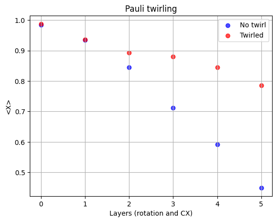
We can clearly see that the twirled circuit yields an expectation value closer to the ideal $\langle X \rangle = 1$. This example served its purpose, but let's move onto something more useful: twirling in the production of highly entangled states.

Pauli twirling in GHZ state preparation

The previous example showed a compelling case for Pauli twirling in destroying the coherent accumulation of errors associated with CNOT gates. GHZ state production uses many CNOT gates to produce highly entangled states useful for many quantum computing applications. Let's explore how Pauli twirling helps in this context, with GHZ states of increasing size.

# Imports if not already loaded in previous cells
# from qiskit.transpiler.preset_passmanagers import generate_preset_pass_manager
# from qiskit import QuantumRegister, ClassicalRegister, QuantumCircuit

# Define a GHZ circuit building function, so that we can build GHZ states of increasing size.

def ghz_circuit(n: int) -> QuantumCircuit:
    q = QuantumRegister(n, "q")
    c = ClassicalRegister(n, "c")
    qc = QuantumCircuit(q, c)

    qc.h(q[0])
    for i in range(n - 1):
        qc.cx(q[i], q[i + 1])

    qc.barrier()

    qc.measure(q, c)
    return qc

# Build a test state with 10 qubits to remind ourselves of GHZ structure.

num_qubits = 10

qc_ghz = ghz_circuit(num_qubits)
qc_isa = pm.run(qc_ghz)
qc_ghz.draw("mpl")

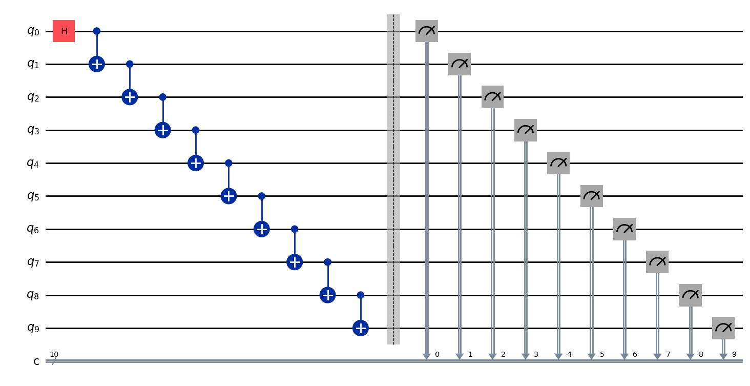
Now we build our circuits and transpile them. In this case, we don't have any artificially repeated gates that reduce to the identity. So we can allow the pass manager to do a bit more optimizing for us. We'll set it to level three.

# Set up a pass manager

opt_level = 3
# --------- Build circuits for a sweep of delays ----------
pm = generate_preset_pass_manager(optimization_level=opt_level, backend=backend)

# Build GHZ circuits of increasing size.

nmin = 5
nmax = 15
circuits = []
for n in range(nmin, nmax):
    qc = ghz_circuit(n)
    qc_isa = pm.run(qc)
    circuits.append(qc_isa)

We can see that the optimizer mapped our abstract circuit to qubits 123, 124, 136, 142, and 143.

circuits[0].draw("mpl")

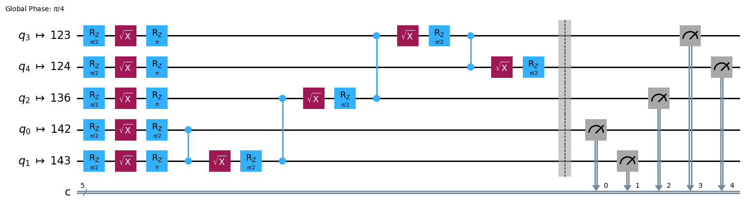
To understand why, let's look at a map of the layout of our backend (in this image, ibm_fez, but you can do equivalent analyses on any backend).

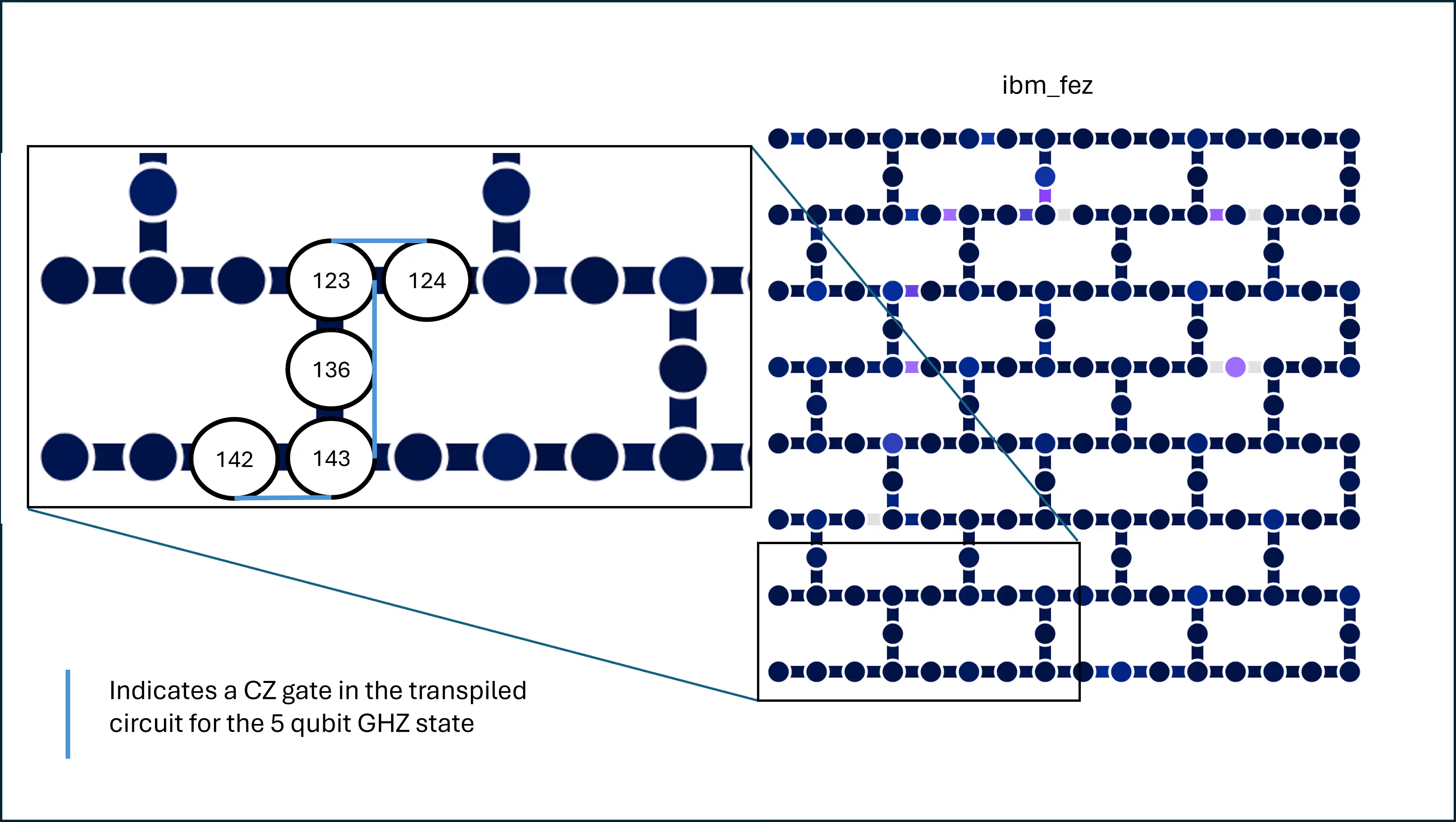
We see that the qubits were selected in a chain to minimize swap gates and thus circuit depth. Further, each CZ gate implemented in the circuit is between adjacent qubits. Finally, all five qubits have relatively low error rates, including readout-assignment error rates. You can check these error rates on any backend on the Compute resources page. Finding such a layout is not difficult for a simple linear chain, but as problems become more complex, the optimization of the circuit layout becomes more difficult and more valuable.

Now we configure our Sampler primitive. We turn off other suppression/mitigation tools to focus on Pauli twirling.

# Configure two Samplers: (A) no twirling, (B) gate twirling
# No DD, no measurement twirling in both (to isolate gate twirling)

shots = 8192

# (A) No twirling
sampler_no_twirl = Sampler(mode=backend)
# Ensure no extra suppression/mitigation:
sampler_no_twirl.options.dynamical_decoupling.enable = False
# Be explicit about twirling:
sampler_no_twirl.options.twirling.enable_gates = False
sampler_no_twirl.options.twirling.enable_measure = (
    False  # TREX-style measurement twirling off
)
sampler_no_twirl.options.default_shots = shots  # default shots for this primitive

# (B) Gate twirling ON
sampler_twirl = Sampler(mode=backend)
sampler_twirl.options.dynamical_decoupling.enable = False
sampler_twirl.options.twirling.enable_gates = True  # <-- enable Pauli gate twirling
sampler_twirl.options.twirling.enable_measure = False
sampler_twirl.options.default_shots = shots

# (Optional) Inspect options dicts if you’re curious
# print(asdict(sampler_no_twirl.options))
# print(asdict(sampler_twirl.options))

Finally, we run our jobs. You can optionally print the job ID numbers for later retrieval.

job = sampler_twirl.run(circuits)
res_ghz_twirl = job.result()
job_id = job.job_id()  # job id for twirling on/true
print("job number for twirling the ghz prep is ", job_id)

job = sampler_no_twirl.run(circuits)
res_ghz_no_twirl = job.result()
job_id = job.job_id()  # job id for twirling off/false
print("job number for NO twirling the ghz prep is ", job_id)

job number for twirling the ghz prep is  d7h967bjne2c7393s0b0
job number for NO twirling the ghz prep is  d7h96f7b91ec73aufing

We extract the counts of each computational basis state measured for all the circuits, both with and without twirling.

# --------- Extract counts per circuit ----------
def extract_counts_list(res):
    counts_list = []
    for r in res:  # each r corresponds to one circuit
        # r.data.<classical_register_name>.get_counts()
        counts = r.data.c.get_counts()
        counts_list.append(counts)
    return counts_list

counts_list_ghz_twirl = extract_counts_list(res_ghz_twirl)
counts_list_ghz_no_twirl = extract_counts_list(res_ghz_no_twirl)

print(counts_list_ghz_twirl[0])
print(counts_list_ghz_twirl[4])

{'11111': 3440, '11101': 87, '00000': 3434, '10111': 87, '00001': 168, '10011': 4, '11000': 102, '00011': 39, '01111': 93, '00111': 111, '01000': 90, '11110': 235, '00110': 6, '00010': 75, '11011': 30, '11100': 42, '10000': 82, '00101': 7, '10001': 2, '11001': 6, '11010': 5, '01010': 3, '01110': 7, '00100': 14, '10101': 1, '10110': 8, '01001': 6, '10100': 1, '01101': 4, '01011': 1, '10010': 2}
{'111111111': 2683, '000000000': 2976, '111000000': 53, '110000000': 74, '111111100': 47, '111011111': 76, '111111110': 195, '111111000': 67, '000000010': 66, '011111110': 10, '011110001': 1, '101110111': 7, '101011111': 9, '111110111': 87, '111100000': 96, '111011000': 2, '010000000': 60, '111111010': 3, '100000000': 110, '111111011': 32, '000000111': 51, '000100000': 84, '000011111': 82, '000000001': 176, '100000010': 6, '111100001': 3, '000000011': 36, '101111111': 98, '100000011': 2, '001111111': 75, '000001000': 60, '000011101': 4, '110111111': 38, '111111101': 72, '111100100': 3, '000100010': 1, '001011101': 1, '000000110': 8, '110000011': 1, '000111111': 48, '000000100': 23, '000001111': 65, '010000101': 2, '000100001': 8, '111110000': 51, '010001111': 1, '111000111': 2, '111000001': 2, '000111100': 1, '011111111': 116, '111110001': 1, '000011110': 10, '000010000': 23, '000101111': 3, '000101110': 1, '011110111': 4, '010000111': 7, '111101111': 36, '001000000': 40, '010100000': 3, '101111110': 8, '110111000': 5, '000000101': 8, '010000010': 4, '000110001': 2, '110111110': 4, '111100010': 2, '111010111': 2, '000001110': 5, '111110101': 3, '001110000': 4, '101100000': 5, '001111110': 8, '100000001': 5, '111011110': 3, '111110100': 5, '110001011': 1, '001110111': 4, '000010110': 2, '111001111': 2, '000011000': 5, '010111110': 1, '000101000': 4, '101000000': 4, '100111111': 4, '111110011': 2, '000101100': 1, '101111100': 2, '111011100': 1, '001111011': 3, '011111011': 3, '110100000': 5, '000001011': 3, '111110110': 5, '111111001': 5, '000001001': 8, '010000001': 5, '011111101': 2, '001010111': 1, '011101110': 1, '110110110': 1, '001111100': 3, '100001000': 3, '001000011': 1, '001011111': 6, '110000010': 2, '110010000': 1, '010011111': 2, '111101101': 3, '101110000': 1, '111100111': 6, '010111111': 5, '110110000': 2, '011011111': 2, '110011111': 1, '110000111': 6, '001000001': 2, '001100000': 3, '101101111': 1, '000111110': 5, '111011101': 2, '100100000': 2, '101111101': 3, '001001111': 1, '001010000': 2, '111001000': 1, '011110000': 2, '011101111': 3, '000001100': 1, '110101000': 1, '011000000': 4, '111101000': 3, '110000001': 4, '000010111': 4, '011111100': 1, '111000010': 1, '101011000': 1, '101111000': 2, '001101111': 1, '010001100': 1, '000100011': 1, '111110010': 1, '111101110': 1, '100001111': 1, '100011011': 1, '010110111': 1, '001110110': 2, '100000100': 1, '001000110': 1, '100011111': 2, '010010001': 1, '111010110': 1, '011110110': 1, '000111000': 2, '000100111': 1, '011010000': 1, '001111000': 2, '100010000': 1, '011111000': 2, '110111100': 2, '110110111': 1, '110001000': 1, '000110111': 1, '000101011': 1, '000110000': 1, '011100000': 3, '001000010': 1, '001001000': 1, '001000111': 1, '001111101': 3, '111101011': 1, '111010000': 1, '100000101': 1, '000010010': 1, '001011110': 1, '000011011': 1, '111101100': 1}

We know the ideal distribution of a GHZ state is that in which half the shots return $|0\rangle^{\otimes N}$ and the other half return $|1\rangle^{\otimes N}$. Build this for comparison.

ideal_dist = []
for n in range(nmin, nmax):
    ideal_dist.append({"0" * n: int(shots / 2), "1" * n: int(shots / 2)})

We now use the Hellinger fidelity as a measure of the quality of our final state.

from qiskit.quantum_info import hellinger_fidelity

num_qubits = []
fidelities_twirl = []
fidelities_no_twirl = []
for n in range(len(ideal_dist)):
    num_qubits.append(nmin + n)
    fidelities_twirl.append(hellinger_fidelity(counts_list_ghz_twirl[n], ideal_dist[n]))
    fidelities_no_twirl.append(
        hellinger_fidelity(counts_list_ghz_no_twirl[n], ideal_dist[n])
    )

Finally we plot our results.

import matplotlib.pyplot as plt

fig, ax = plt.subplots()

# Add values using no twirling
ax.scatter(
    num_qubits,
    fidelities_no_twirl,
    c="blue",
    linestyle="-",
    label="No twirl",
    alpha=0.7,
)

## Add values with twirling
ax.scatter(
    num_qubits, fidelities_twirl, c="red", linestyle="-", label="Twirled", alpha=0.7
)

# Add labels and plot
ax.set_xlabel("Qubits in GHZ state")
ax.set_ylabel("Hellinger fidelity")
ax.legend()
ax.set_title("Pauli twirling in GHZ states")
ax.grid(True)

plt.show()

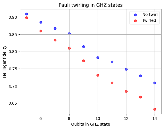
The results using Pauli twirling are no better (and even slightly worse) than without twirling. What happened?

Two things happened. First, Pauli twirling does not reduce the total amount of noise — rather, it reshapes coherent, systematic errors into stochastic Pauli‑type errors, so that error growth becomes predictable and modelable. There was never any promise of error reduction, except in special cases.

Secondly, in GHZ circuits, some coherent errors can partially cancel or act like benign phase shifts because of the symmetry of the GHZ construction; twirling removes this accidental protection and replaces it with uncorrelated stochastic Pauli noise, so GHZ fidelity becomes slightly worse under twirling.

This second claim requires some explanation. The claim is not that GHZ circuits are protected from all kinds of coherent error accumulation, only some kinds — and that in those cases the protection is destroyed by twirling. Specifically, let's consider coherent over-rotation associated with the CX gates. Let us call the real CX gate with over-rotation $\tilde{CX}$:

$$\tilde{CX}\equiv e^{-i\epsilon K} \cdot CX$$

where $K$ is any product of Pauli operators, like $X$, $Z$, $Z \otimes X$, $Z^{\otimes N}$, etc. For general states, any of these over-rotations could affect measurement statistics (and thus measures of state fidelity). A subset of these, however, leaves many standard GHZ observables unchanged, including operators such as $Z_i Z_j$ and $Z^{\otimes N}$. In the context of preparing a GHZ state, the relevant over-rotation errors of this type would be:

$$\tilde{CX}\equiv e^{-i\epsilon Z_c Z_t} \cdot CX$$

The preparation of the entire $N$-qubit GHZ state would look like:

$$|\psi_\text{GHZ}\rangle=\prod_{j=0}^{N-2}{e^{-i\epsilon Z_j Z_{j+1}} \cdot CX_{j,j+1}}H^{\otimes N}|0^{\otimes N}\rangle$$

After preparing the GHZ state, the state is ideally:

$$|\text{GHZ}^{\otimes N}\rangle=\frac{1}{\sqrt{2}}\left(|0\dots 0\rangle + |1\dots 1\rangle\right).$$

This state is a simultaneous eigenstate of a large set of Pauli operators, including the following:

$$Z_i Z_j \quad \text{for all } i \neq j,$$

with eigenvalue $+1$. As a result, an operator of the form $e^{-i\epsilon Z_i Z_j}$ acts on the GHZ state as multiplication by the phase factor $e^{-i\epsilon}$, which does not affect standard GHZ observables such as parity, collective $X^{\otimes N}$, or computational‑basis populations. Thus, although the over‑rotation errors $e^{-i\epsilon Z_j Z_{j+1}}$ are coherent and systematic, they are effectively invisible to the measurements used to assess GHZ fidelity. In this sense, the GHZ circuit enjoys an accidental coherence protection: certain coherent CX errors commute with the structure of the state being prepared and therefore do not degrade measured performance.

Pauli twirling fundamentally changes this situation. Twirling does not preserve the coherent over‑rotation error as a deterministic $Z_jZ_{j+1}$ process. Instead, it converts the coherent error channel into an effective stochastic Pauli channel. As a result, the error channel now includes terms such as $X$, $Y$, $X \otimes Z$, and $Y \otimes X$, which do not commute with the GHZ stabilizers.

When these stochastic Pauli errors occur, they create real bit‑flip and phase‑flip faults on individual qubits or pairs of qubits. These errors take the state out of the GHZ stabilizer subspace, reduce interference between $|0\dots 0\rangle$ and $|1\dots 1\rangle$, and directly lower GHZ fidelity and multi‑qubit parity signals. In other words, Pauli twirling removes the coherent structure of the error but also removes the symmetry‑based cancellation that previously made those errors benign. The result is a slightly worse GHZ state — not because twirling adds noise, but because it converts a mostly harmless coherent error into genuinely damaging stochastic errors.

This example highlights an important lesson: Pauli twirling is not a universal improvement strategy. It is most beneficial when coherent errors accumulate across a circuit in a manner destructive to the required fidelity. In highly symmetric circuits like GHZ state preparation, some coherent errors are naturally aligned with the state’s stabilizers, and deliberately randomizing them can eliminate this accidental protection.

Combine methods

One can in principle combine Pauli twirling with dynamical decoupling. We have not used DD in this case for two reasons: firstly there should not be any extremely long idle periods in this circuit. Secondly, GHZ states do not store most of their information in single-qubit phase coherence, particularly if we are observing the fidelity only in terms of bitstring counts, and not in terms of the phase between the desired bitstrings $|0\rangle^{\otimes N}$ and $|1\rangle^{\otimes N}$.

If we were to extend the GHZ preparation to 100+ qubits, then the delays in measuring the first/early qubits might indeed be long enough that DD could be useful. This is especially true when we take into account the transpiled depth of the circuit.

Pauli twirling in RTZ echo structure

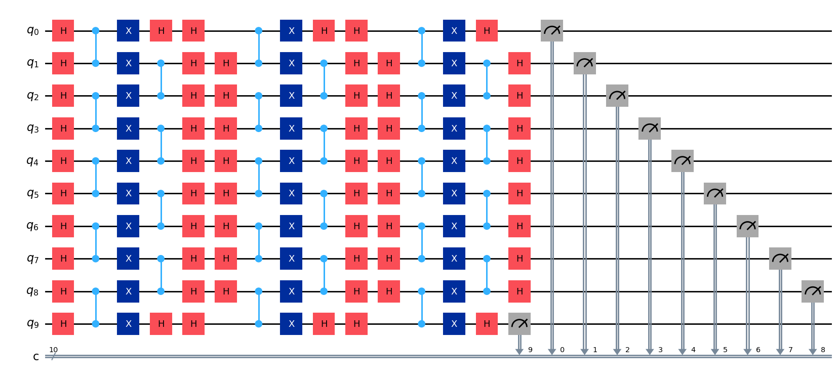
Our final example of Pauli twirling in the context of reducing coherent error accumulation uses a circuit with layers of X-CZ-X-CZ combinations. This is a well-known gate sequence that is often used to cancel coherent ZZ error terms in two-qubit gates, even without twirling. But with twirling, we can reduce or randomize other forms of coherent error accumulation.

We'll start by defining a function to build the RTZ-like circuits with a varying number of layers.

from qiskit import QuantumCircuit

def rtz_echo_circuit(n_qubits: int, depth: int) -> QuantumCircuit:
    """
    Construct an RTZ echo-style circuit.

    Args:
        n_qubits: Number of qubits in the circuit.
        depth: Number of repeated echo layers.

    Returns:
        A QuantumCircuit implementing the echo sequence with measurements.
    """
    q = QuantumRegister(n_qubits, "q")
    c = ClassicalRegister(n_qubits, "c")
    qc = QuantumCircuit(q, c)

    for _ in range(depth):
        qc.h(q)

        for i in range(0, n_qubits - 1, 2):
            qc.cz(q[i], q[i + 1])

        qc.x(q)

        for i in range(1, n_qubits - 1, 2):
            qc.cz(q[i], q[i + 1])

        qc.h(q)

    qc.measure(q, c)
    return qc

Now we build circuits with increasing layers, up to some reasonable total transpiled two-qubit depth.

from qiskit.transpiler.preset_passmanagers import generate_preset_pass_manager

circuits = []
qcs = []
depths = list(range(3, 27, 4))
n_qubits = 10

opt_level = 0
pm = generate_preset_pass_manager(
    optimization_level=opt_level,
    backend=backend,
    initial_layout=[0, 1, 2, 3, 4, 5, 6, 7, 8, 9],
)

for d in depths:
    qc = rtz_echo_circuit(n_qubits, d)
    qcs.append(qc)
    qc_isa = pm.run(qc)
    circuits.append(qc_isa)

# We can check the 2-qubit depths of any of our circuits like this:
two_qubit_depths = []
for n in range(len(circuits)):
    two_qubit_depths.append(
        circuits[n].decompose().depth(lambda instr: len(instr.qubits) > 1)
    )
print(two_qubit_depths)

[6, 14, 22, 30, 38, 46]

qcs[0].draw("mpl")
# circuits[0].draw("mpl")

At the high end, some of these are quite deep. Let's use the AerSimulator with no noise model to obtain the ideal states at the end of each of these circuits. We can then can benchmark our results from real quantum computers using the Hellinger fidelity.

from qiskit_aer import AerSimulator

sim = AerSimulator()
ideal_results = sim.run(circuits, shots=8192).result()
ideal_counts = ideal_results.get_counts()

Now we define a SamplerV2 with twirling, and one without twirling.

from qiskit_ibm_runtime import SamplerV2 as Sampler

shots = 8192

# --- No Twirling ---
sampler_no = Sampler(mode=backend)
sampler_no.options.twirling.enable_gates = False
sampler_no.options.twirling.enable_measure = False
sampler_no.options.default_shots = shots

# --- With Twirling ---
sampler_tw = Sampler(mode=backend)
sampler_tw.options.twirling.enable_gates = True
sampler_tw.options.twirling.enable_measure = False
# sampler_tw.options.twirling.num_randomizations = "auto"
sampler_tw.options.twirling.num_randomizations = 32
sampler_tw.options.twirling.strategy = "active-circuit"
sampler_tw.options.default_shots = shots

Now we run our jobs.

# Each job took 17 sec (34 sec total) on ibm_fez. Your times might vary.

job_no = sampler_no.run(circuits)
job_tw = sampler_tw.run(circuits)

res_no = job_no.result()
res_tw = job_tw.result()

We get the counts from each of the runs on a real quantum computer.

counts_no = [r.data.c.get_counts() for r in res_no]
counts_tw = [r.data.c.get_counts() for r in res_tw]

Now we find the Hellinger fidelity by comparing each of these runs to the noise-free AerSimulator results.

from qiskit.quantum_info import hellinger_fidelity

f_no = [hellinger_fidelity(counts_no[i], ideal_counts[i]) for i in range(len(circuits))]

f_tw = [hellinger_fidelity(counts_tw[i], ideal_counts[i]) for i in range(len(circuits))]

Now we visualize our results.

import matplotlib.pyplot as plt

plt.figure(figsize=(8, 5))
plt.plot(two_qubit_depths, f_no, "o-", label="No Twirling")
plt.plot(two_qubit_depths, f_tw, "o-", label="With Twirling")
plt.xlabel("Two-qubit transpiled depth")
plt.ylabel("Hellinger Fidelity")
plt.title("RTZ Echo Circuit: Twirling vs No Twirling")
plt.legend()
plt.grid(True)
plt.show()

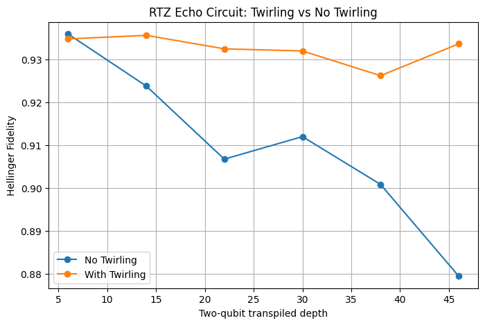
Throughout this lesson, we have examined cases in which Pauli twirling is used to limit coherent error accumulation, a context in which it might be described as error suppression. However, Pauli twirling is often more useful as a tool for reshaping error behavior, converting coherent errors into a form that is more predictable and easier to model. The usefulness of this will become more apparent in the context of error-mitigation techniques such as zero-noise extrapolation (ZNE), which rely on reasonably predictable noise scaling. This is discussed in the next lesson.