Rimay Quantum Feature Extraction - a Qiskit Function by Kipu Quantum

note

Qiskit Functions are an experimental feature available only to IBM Quantum® Premium Plan, Flex Plan, and On-Prem (through the IBM Quantum Platform API) Plan users. They are in preview release status and subject to change.

Overview

Rimay augments classical machine learning pipelines with features generated on quantum hardware. The function takes classical tabular data and returns a set of quantum-transformed features. When a quantum system processes the data, it generates rich features that capture nonlinear relationships between the inputs. You can use the generated features on their own, or combined with your original features, to train any classical model. On small- and medium-sized datasets, quantum-transformed features can improve the prediction quality compared to purely classical baselines.

This function is built for the following users:

Data science teams with an existing machine learning pipeline on small- and medium-sized tabular datasets, where prediction quality has plateaued. You add Rimay as one additional preprocessing step, without building any quantum circuits yourself.
Researchers who explore quantum methods for machine learning tasks.

Description

The quantum feature extraction algorithm [1] combines two principles of quantum machine learning. The first is quantum feature maps, which embed data into a high-dimensional Hilbert space and therefore produce more expressive representations. The second is quantum reservoir computing, which uses the dynamics of a quantum many-body system as a nonlinear transformation of the input.

Rimay encodes the feature values and the mutual information between the features into the local fields and the coupling coefficients of a spin-glass Hamiltonian. Counterdiabatic quantum dynamics evolve the system toward its low-energy states, which contain nonlinear mixtures of the correlations in the input data. Rimay extracts these correlations by measuring single- and two-body expectation values. The expectation values are the quantum-transformed features that you feed into your machine learning model.

Workflow

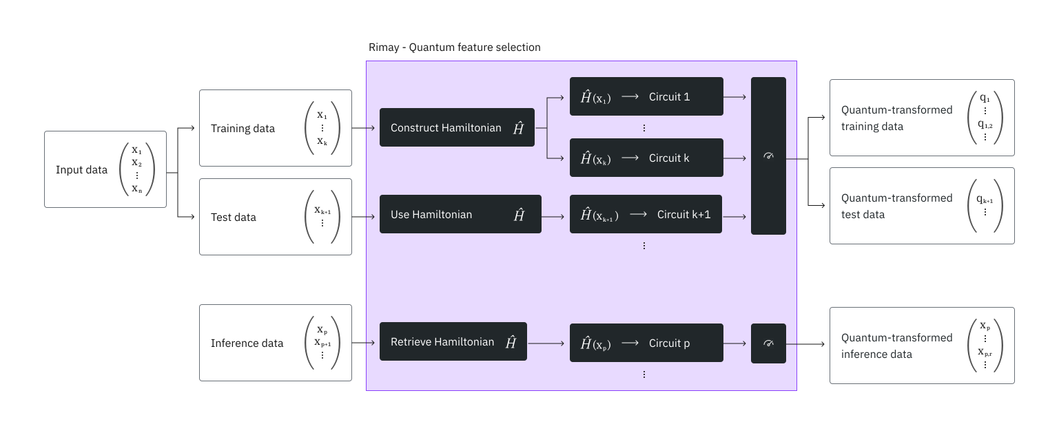
Rimay workflow: The training data defines the Hamiltonian, every sample becomes one circuit, and the measured expectation values are returned as quantum-transformed data

Preprocess your tabular data as you would for classical machine learning. Rimay needs numerical features, so convert categorical features into numerical ones, for example with scikit-learn's OneHotEncoder.
Split the data into a training set and a test set, and upload both to the function, as shown in the Example section.
Rimay uses the training data to construct the Hamiltonian that represents the data. Every feature corresponds to one qubit, and the full training set decides which features, and therefore which qubits, interact. Rimay stores this structure so that it maps the test data and later inference data with the same Hamiltonian.
For every sample, the feature values set the local fields of the Hamiltonian, and the mutual information between the features sets the coupling coefficients of the structure from step 3. Rimay digitizes the counterdiabatic evolution of this Hamiltonian into a circuit, and runs the circuits on the QPU.
Rimay measures the resulting bitstrings, then computes the single-body expectation values and the two-body expectation values of physically coupled qubits.
You download the expectation values in a form that you can feed directly into your model, or combine with your original features.

note

Because of this structure, the number of qubits that a run needs equals the number of features, and the number of circuits that it submits equals the number of samples.

After you fit a mapping, you can map new data through it, for example for inference. Rimay then retrieves the Hamiltonian that it created during the fit and builds the circuits for the new samples from it.

Integrate Rimay into your machine learning pipeline

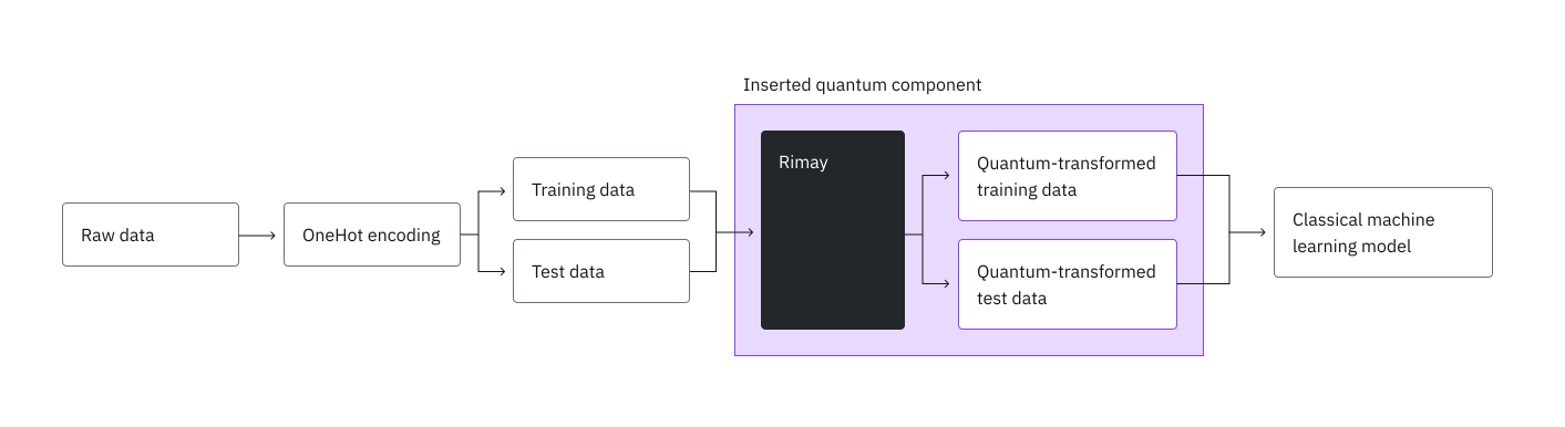
Pipeline with Rimay inserted between the train-test split and the classical machine learning model

As in a classical pipeline, you start by preprocessing the raw data, for example by one-hot encoding the categorical features, and split it into a training set and a test set. Instead of feeding both sets into your model directly, you feed them into Rimay first, and train your model on the quantum-transformed features.

Benchmarks

Kipu Quantum benchmarked Rimay on the German credit dataset from OpenML [2], which classifies 1000 credit applicants as good or bad credit risks. It has 13 categorical and seven numerical attributes. One-hot encoding of the categorical attributes results in 48 numerical features. The benchmark holds out 20% of the samples as the test set.

As a baseline, several classical models were trained on the classical features. With Rimay, a random forest was trained in two ways: on the quantum-transformed features alone (Random forest Q), and on the quantum-transformed features combined with the classical ones (Random forest H, for hybrid). The table reports only the random forest, because it performed best on the quantum-transformed features.

Model	Features	Accuracy	AUC	F1 score	Precision	Recall
CatBoost	Classical	0.775	0.781	0.850	0.795	0.914
Random forest	Classical	0.765	0.781	0.846	0.782	0.921
XGBoost	Classical	0.760	0.758	0.835	0.803	0.871
LightGBM	Classical	0.770	0.751	0.840	0.818	0.864
Random forest Q	Quantum	0.750	0.793	0.840	0.762	0.936
Random forest H	Hybrid	0.770	0.798	0.854	0.770	0.957

The hybrid features improve all metrics of the random forest except the precision, and the hybrid random forest reaches a higher AUC, F1 score, and recall than CatBoost on the classical features. The largest effect is on the recall, which rises from 0.921 to 0.957. The quantum-transformed features alone do not reach the precision of the classical models.

caution

The test set holds only 200 samples, so predicting one more sample correctly moves the accuracy by 0.005. Read the differences as a trend that needs further verification, not as a significant effect. The prediction accuracy can also depend on the hardware-induced noise of the extracted features. Therefore, use enough shots that shot noise does not limit the result.

The benchmark used the following resources:

Example	Number of qubits	Number of samples	Number of shots	Total time (min)	QPU usage (min)	Processor
German credit	48	1000	5000	23	22	ibm_boston
German credit	48	1000	5000	3	2	ibm_phoenix

The number of samples, which is the number of circuits, drives the QPU time. Use the Nighthawk r2 processor type, because it greatly reduces the required QPU time.

Inputs

The mode determines which parameters a run needs. For a description of every input parameter, see the API reference.

Input files

Upload every file with catalog.file_upload() before you run the function.
An upload replaces any earlier file of the same name, even for a job that you submitted but that has not started yet. To run several jobs at the same time, give the files of each job their own names, for example run1_x_train.csv and run2_x_train.csv.
Every file is a CSV file with a header row. Every column of a feature file is one feature, and every value must be numeric.
y_train holds exactly one numeric column, with one label per row of x_train. Map categorical labels to numbers, for example good and bad to 1 and 0.
x_test and x_inference must have the same columns as x_train, in the same order.

Keep the mapping_id and backend_name

The mapping_id is the only way to reach the mapping that your fit produced, and it cannot be looked up or recovered. It authorizes the use of that mapping, so treat it like a credential and do not share it. If you lose it, you must fit a new mapping, which costs another run on quantum hardware. Also record the backend_name of the fit, because the mapping runs only on that processor.

Limits

Every feature is mapped to one qubit, so the processor must have at least as many qubits as your data has features. If you have more features than that, reduce them with a feature selection technique first.
Every sample becomes one circuit, and a run counts training and test samples together. A run can hold at most 15,000 samples.
A single job can request at most 10 million executions, so the number of samples times shots must not exceed 10 million.
A job must finish within 24 hours, including the time its circuits wait in the processor's queue. A job that runs longer is stopped without a result. On a busy processor, keep large datasets well below these limits.

Outputs

job.result() returns a dictionary. The quantum-transformed features themselves are written to CSV files that you download with catalog.file_download(). For a description of every key of the dictionary, see the API reference. For the time that each execution phase took, see Run metadata.

Every output file holds one row per input row, in the order of the input file, and one column per quantum-transformed feature. The columns whose names start with corr_ are the two-body expectation values. The files hold no label column. The labels of your training data stay in your y_train file.

Run metadata

resource_usage holds one entry for each execution phase that the run went through: "RUNNING: MAPPING", "RUNNING: POST_PROCESSING", and, on a QPU, usually "RUNNING: WAITING_FOR_QPU". Each entry holds CPU_TIME, the wall-clock time of the phase in seconds, and QPU_TIME, the QPU time in seconds. On a QPU, the QPU time that IBM billed is recorded under "RUNNING: MAPPING", the phase in which the circuits ran.

"RUNNING: WAITING_FOR_QPU" is the time your jobs waited in the IBM queue. The run takes this time from the IBM job timestamps, and does not count it in "RUNNING: MAPPING". If IBM does not report those timestamps for every job, the entry is absent, and the wait is part of "RUNNING: MAPPING".

IBM® finishes its usage calculation some time after a job finishes. The run waits up to about a minute for it. Usage that is still being calculated after that time is not included in QPU_TIME, and the final usage is shown on IBM Quantum Platform. If the run cannot read the usage from IBM, QPU_TIME is None.

For example:

"metadata": {
    "version": "0.3.0",
    "resource_usage": {
        "RUNNING: MAPPING": {"CPU_TIME": 12.4, "QPU_TIME": 6.0},
        "RUNNING: WAITING_FOR_QPU": {"CPU_TIME": 28.8, "QPU_TIME": 0.0},
        "RUNNING: POST_PROCESSING": {"CPU_TIME": 0.3, "QPU_TIME": 0.0},
    },
}

Get started

Authenticate using your IBM Quantum Platform API key, and select the Qiskit Function as follows:

note

The following code assumes that you have saved your credentials. If you have not, follow the instructions in Install the Qiskit Functions Catalog client to save your account with your API key.

# Added by doQumentation — installs the packages this notebook needs if they are missing
import importlib.util

_needed = {"pandas": "pandas", "qiskit_ibm_catalog": "qiskit-ibm-catalog"}
_missing = [pip for module, pip in _needed.items()
            if importlib.util.find_spec(module) is None]
# One at a time, so a package that fails to install does not block the others
for _pip in _missing:
    %pip install -q {_pip}
if not _missing:
    print("\u2713 All required packages are installed")

from qiskit_ibm_catalog import QiskitFunctionsCatalog

catalog = QiskitFunctionsCatalog(channel="ibm_quantum_platform")

# Verify that you have access to the function
catalog.list()

[QiskitFunction(kipu-quantum/rimay)]

# Access function
rimay = catalog.load("kipu-quantum/rimay")

Function sizes

Every job runs at one size — S, M, or L. If the specified size is too small, the job is rejected. If the size is larger than needed, it runs on a bigger compute profile than the work requires.

The size of a Rimay job depends on the number of samples it maps: the rows of x_train and x_test for fit-transform, and the rows of x_inference for transform. The labels in y_train do not count, and a delete run maps no samples.

Size	Samples per job	Compute profile	vCPU	RAM
`S`	Up to 2,999	`8x32`	8	32 GB
`M`	3,000 to 9,999	`8x32`	8	32 GB
`L`	10,000 to 15,000	`16x128`	16	128 GB

The number of samples is the only criterion. A size changes nothing but the compute profile: the limits on features, samples, and shots are the same for every size. S and M run on the same compute profile and differ in the number of samples each covers.

The default is M, used when a job does not request a size. A job of more than 9,999 samples must therefore request L.

You can also read the mapping off the function itself with rimay.sizes_map, and the size that a job runs at when it does not request one with rimay.default_size.

Calculate the size before submitting

Run this on your own inputs. It reads them and does nothing else: no job is submitted and nothing is reserved, so you can call it as often as you like.

Pass the data sets themselves, not their file names, in the same order as input_file, together with the mode of the run. Step 2 of the example shows the call.

from os import PathLike
from typing import Any, Literal, Sequence, Sized

Size = Literal["S", "M", "L"]

# Upper bounds (inclusive) in samples.
_SMALL = 2_999
_MEDIUM = 9_999

FIT_TRANSFORM, TRANSFORM, DELETE = "fit-transform", "transform", "delete"

# Which positions of input_file hold samples, per mode. The labels in
# y_train submit no circuits of their own, so they are not counted.
SAMPLE_POSITIONS = {FIT_TRANSFORM: (0, 2), TRANSFORM: (0,)}

def calculate_function_size(problem: Sequence[Sized], **kwargs: Any) -> Size:
    """Return the size ("S", "M" or "L") required to run the function."""
    metrics = _measure(problem, **kwargs)
    if _is_small(metrics):
        return "S"
    if _is_medium(metrics):
        return "M"
    return "L"

def _measure(problem: Sequence[Sized], **kwargs: Any) -> dict:
    """The samples the job submits."""
    return {"samples": count_samples(problem, kwargs.get("mode"))}

def count_samples(problem: Sequence[Sized], mode: Any) -> int:
    """Rows across the data sets of ``problem`` that carry samples."""
    if mode == DELETE:
        return 0
    if mode not in SAMPLE_POSITIONS:
        raise ValueError(f"cannot size mode {mode!r}")
    if _is_name(problem) or (
        isinstance(problem, (list, tuple))
        and any(_is_name(data) for data in problem)
    ):
        raise TypeError(
            "pass the data, not the file name: read each input_file, e.g. with "
            "pandas.read_csv, and pass the data sets in input_file order"
        )
    if not isinstance(problem, (list, tuple)):
        raise TypeError(
            "pass a list of data sets in input_file order, e.g. [x_train, y_train], "
            f"not a single {type(problem).__name__}"
        )
    return sum(
        len(problem[i]) for i in SAMPLE_POSITIONS[mode] if i < len(problem)
    )

def _is_name(value: Any) -> bool:
    """A file name or path rather than data."""
    return isinstance(value, (str, bytes, PathLike))

def _is_small(metrics: dict) -> bool:
    """Determine if the metrics fit T-size 'S'."""
    return metrics["samples"] <= _SMALL

def _is_medium(metrics: dict) -> bool:
    """Determine if the metrics fit T-size 'M'."""
    return metrics["samples"] <= _MEDIUM

If the size is too small, the job fails with error 4600 and the message names the size to use instead. If it is larger than needed, the job runs normally and records a 4601 advisory event.

Example

This example shows how to upload data, run the function, and retrieve the quantum-transformed features. For an end-to-end example that includes the preprocessing and the training of the classical model, see the tutorial.

1. Upload the data

This example uses a small synthetic dataset with four numeric features and a binary label, so that a run needs only four qubits and finishes quickly. The next cell writes it to four CSV files: the training features, the training labels, the test features, and the features for step 4 of this example. To use your own data, write your preprocessed training and test sets to files with the same layout instead.

from pathlib import Path

Path("x_train.csv").write_text("""f0,f1,f2,f3
7227,1.3355,1.9595,2.5562
2731,0.5779,0.8983,1.1624
1139,0.1817,0.2163,0.2426
0341,0.1311,0.0854,0.09
8996,1.6951,2.497,3.3407
9669,1.8906,2.7705,3.6569
6366,1.2821,1.8793,2.4602
7718,1.4979,2.2223,2.933
5465,1.1008,1.67,2.2195
9475,1.9423,2.8942,3.8199
8829,1.6842,2.4703,3.2865
0675,0.0365,0.0705,0.0162
""")
Path("y_train.csv").write_text("label\n1\n0\n0\n0\n1\n1\n0\n1\n0\n1\n1\n0\n")
Path("x_test.csv").write_text("""f0,f1,f2,f3
543,1.0786,1.5684,2.0607
9928,1.9037,2.9302,3.8422
2269,0.3637,0.4628,0.597
9896,1.9511,2.8913,3.8208
""")
Path("x_inference.csv").write_text("""f0,f1,f2,f3
2708,0.542,0.8506,1.0897
3585,0.6025,0.9517,1.2609
8871,1.6559,2.4577,3.2992
""")

Upload the training and test files. You upload x_inference.csv in step 4.

for file_name in ("x_train.csv", "y_train.csv", "x_test.csv"):
    catalog.file_upload(file_name, rimay)

2. Run the function

Calculate the size of the run from the data that you uploaded, with the calculator from Function sizes.

import pandas as pd

x_train = pd.read_csv("x_train.csv")
y_train = pd.read_csv("y_train.csv")
x_test = pd.read_csv("x_test.csv")

size = calculate_function_size(
    [x_train, y_train, x_test], mode="fit-transform"
)
print(size)

Select a processor with at least as many qubits as your data has features, and run the function in fit-transform mode with that size. The sample data has four features, so any IBM Quantum processor can run it.

backend = catalog.least_busy(operational=True, simulator=False)

job = rimay.run(
    mode="fit-transform",
    input_file=["x_train.csv", "y_train.csv", "x_test.csv"],
    backend_name=backend.name,
    shots=5000,
    function_size=size,
)
print(job.job_id)

85dabc9f-a769-4f4a-8e92-f3be73f85ca2

Check the workload's status or return results as follows:

# Monitor the job status
job.status()

'DONE'

result = job.result()

# Keep both: the mapping_id is the only handle on the mapping this run
# fitted, and the mapping runs only on the processor it was fitted on.
mapping_id = result["mapping_id"]
fit_backend_name = result["backend_name"]

3. Retrieve the results

Download the quantum-transformed features. Pass target_name so that each file is saved under its own name.

for file_name in result["output_files"]:
    catalog.file_download(file_name, rimay, target_name=file_name)

693iB [00:00, 171kiB/s]
254iB [00:00, 111kiB/s]

4. Map new data

After you train your model, map new data with the fitted mapping, for example to run inference. This example maps x_inference.csv, which the first cell of this example wrote. Pass the mapping_id that the fit returned, so that the new rows are mapped with the same mapping instead of a new one.

A mapping is built for the qubit layout of one processor, so pass the same backend_name as the fit, which the fit returned in result["backend_name"]. Do not use least_busy() to choose the processor, because it might return a different one. Rimay rejects any other processor before it submits anything. The shot count also comes from the fit.

catalog.file_upload("x_inference.csv", rimay)

x_inference = pd.read_csv("x_inference.csv")
size = calculate_function_size([x_inference], mode="transform")

job = rimay.run(
    mode="transform",
    input_file=["x_inference.csv"],
    # The processor the mapping was fitted on
    backend_name=fit_backend_name,
    shots=5000,
    mapping_id=mapping_id,
    function_size=size,
)

# Monitor the job status
job.status()

'DONE'

result = job.result()

for file_name in result["output_files"]:
    catalog.file_download(file_name, rimay, target_name=file_name)

202iB [00:00, 73.5kiB/s]

5. Delete a mapping

When you no longer need a fitted mapping, delete it. A delete run does no quantum work, so it needs no processor, no shots, and no function size. You cannot undo a deletion. After deletion, the mapping_id no longer refers to anything, and a transform run with it fails.

job = rimay.run(mode="delete", mapping_id=mapping_id)
job.result()

{'output_files': [],
 'mode': 'delete',
 'deleted': True,
 'mapping_id': '30L40joyUPYfnvgwo2d7MXXSzqvHkggR-Kzn81wfIYw',
 'metadata': {'version': '0.6.0', 'resource_usage': {}}}

Fetch error messages

If your workload status is ERROR, use job.error_message() to fetch the error message, as follows:

job = rimay.run(
    mode="fit-transform",
    input_file=["x_train.csv", "y_train.csv"],
    backend_name=backend.name,
    shots=0,
)
job.error_message()

Every error that Rimay reports carries a code from the IBM Quantum error codes, a message, and a solution that names the value that you passed and the value that is allowed. The following table lists the most common errors:

Code	Cause
`1221`	A parameter is missing or has the wrong type, `mode` is not valid, a file named in `input_file` was not uploaded, the files do not match each other, a feature is not numeric, or the `mapping_id` does not match a stored mapping.
`1221`	A `"transform"` run names a different `backend_name` than the fit that produced its mapping.
`1216`	Your instance has no processor with the `backend_name` that you passed. The solution lists the processors it does have.
`1200`	Your API key does not have access to the instance that the job runs under.
`3200`	`backend_name` does not start with `ibm_`.
`4500`	The data has more features than the processor has qubits.
`6000`	The number of samples times `shots` exceeds 10 million executions.
`6001`	`shots` is smaller than 1.
`6002`	The data has more samples than a run allows.

Use cases

In tabular classification on small- and medium-sized datasets, Kipu Quantum has applied quantum feature extraction to the following:

Beyond tabular data, frozen neural networks can transform images into numerical features, which quantum feature extraction then maps into quantum-transformed features:

Satellite image classification [3]

Get support

For support, contact support@kipu-quantum.com.

Next steps

Visit the API reference for this Qiskit Function.
Try the Classify credit risk with Kipu Quantum's Rimay quantum feature extraction tutorial.
Review Simen, A., et al. (2025). Digitized Counterdiabatic Quantum Feature Extraction. arXiv preprint arXiv:2510.13807.
Review Zhang, Q., et al. (2026). Quantum-enhanced satellite image classification. arXiv preprint arXiv:2602.18350.

References

[1] Simen, A., et al. (2025). Digitized Counterdiabatic Quantum Feature Extraction. arXiv preprint arXiv:2510.13807.

[2] Hofmann, H. (1994). Statlog (German Credit Data). OpenML dataset 31.

[3] Zhang, Q., et al. (2026). Quantum-enhanced satellite image classification. arXiv preprint arXiv:2602.18350.

Additional information

Rimay is a Quechua word that means "to explain".

Overview​

Description​

Workflow​

Integrate Rimay into your machine learning pipeline​

Benchmarks​

Inputs​

Input files​

Limits​

Outputs​

Run metadata​

Get started​

Function sizes​

Calculate the size before submitting​

Example​

1. Upload the data​

2. Run the function​

3. Retrieve the results​

4. Map new data​

5. Delete a mapping​

Fetch error messages​

Use cases​

Get support​

Next steps​

References​

Additional information​

Overview

Description

Workflow

Integrate Rimay into your machine learning pipeline

Benchmarks

Inputs

Input files

Limits

Outputs

Run metadata

Get started

Function sizes

Calculate the size before submitting

Example

1. Upload the data

2. Run the function

3. Retrieve the results

4. Map new data

5. Delete a mapping

Fetch error messages

Use cases

Get support

Next steps

References

Additional information