Optimization Solver: A Qiskit Function by Q-CTRL Fire Opal

See the API reference

note

Qiskit Functions are an experimental feature available only to IBM Quantum® Premium Plan, Flex Plan, and On-Prem (via IBM Quantum Platform API) Plan users. They are in preview release status and subject to change.

Package versions

The code on this page was developed using the following requirements. We recommend using these versions or newer.

qiskit-ibm-runtime~=0.47.0
sympy~=1.14.0

Overview

With the Fire Opal Optimization Solver, you can solve utility-scale optimization problems on quantum hardware without requiring quantum expertise. Simply input the high-level problem definition, and the Solver takes care of the rest. The entire workflow is noise-aware and leverages Fire Opal's Performance Management under the hood. The Solver consistently delivers accurate solutions to classically challenging problems, even at full-device scale on the largest IBM® QPUs.

The Solver is flexible and can be used to solve combinatorial optimization problems defined as objective functions or arbitrary graphs. Problems do not have to be mapped to device topology. Both unconstrained and constrained problems are solvable, with constraints enforced as hard Hamming-weight-1 constraints rather than penalty terms. The examples included in this guide demonstrate how to solve an unconstrained and a constrained utility-scale optimization problem using different Solver input types. The first example involves a max-cut problem defined on a 156-node, 3-Regular graph, while the second example tackles a 50-node graph partitioning problem defined by a cost function.

To get access to the Optimization Solver, contact Q-CTRL.

Function description

The Solver fully optimizes and automates the entire algorithm, from error suppression at the hardware level to efficient problem mapping and closed-loop classical optimization. Behind the scenes, the Solver's pipeline reduces errors at every stage, enabling the enhanced performance required to meaningfully scale. The underlying workflow is inspired by the Quantum Approximate Optimization Algorithm (QAOA), which is a hybrid quantum-classical algorithm. For a detailed summary of the full Optimization Solver workflow, refer to the published manuscript.

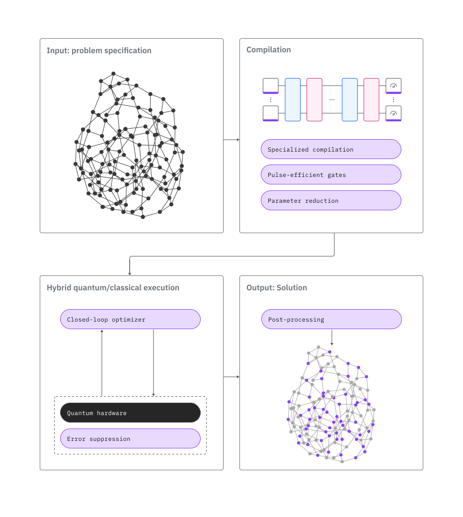
To solve a generic problem with the Optimization Solver:

1. Define your problem as an objective function, a graph, or SparsePauliOp spin chain.
2. Connect to the function through the Qiskit Functions Catalog.
3. Run the problem with the Solver and retrieve results.

Accepted problem formats

• Polynomial expression representation of an objective function. Ideally created in Python with an existing SymPy Poly object and formatted into a string using sympy.srepr.
• Graph representation of a specific problem type. The graph should be created using the networkx library in Python. It should then converted to a string by using the networkx function nx.readwrite.json_graph.adjacency_data.
• Spin chain representation of a specific problem. The spin chain should be represented as a SparsePauliOp object; see the documentation for more details.

Does this function support all IBM backends?

If you want to use a backend that this function does not currently support, reach out to Q-CTRL to add support.

Benchmarks

Published benchmarking results show that the Solver successfully solves problems with over 120 qubits, even outperforming previously published results on quantum annealing and trapped-ion devices. The following benchmark metrics provide a rough indication of the accuracy and scaling of problem types based on a few examples. Actual metrics may differ based on various problem features, such as the number of terms in the objective function (density) and their locality, number of variables, and polynomial order.

The "Number of qubits" indicated is not a hard limitation but represents rough thresholds where you can expect extremely consistent solution accuracy. Larger problem sizes have been successfully solved, and testing beyond these limits is encouraged.

Arbitrary qubit connectivity is supported across all problem types.

Problem type	Number of qubits	Example	Accuracy	Total time (s)	Runtime usage (s)	Number of iterations
Sparsely-connected quadratic problems	156	3-regular max-cut	100%	1764	293	16
Higher-order binary optimization	156	Ising spin-glass model	100%	1461	272	16
Densely-connected quadratic problems	50	Fully-connected max-cut	100%	1758	268	12
Constrained problem with hard constraints	50	Weighted graph partitioning with 8% edge density	100%	1074	215	10

Get started

First, authenticate using your IBM Quantum API key. Then, select the Qiskit Function as follows. (This snippet assumes you've already saved your account to your local environment.)

# Added by doQumentation — required packages for this notebook
!pip install -q networkx numpy qiskit-ibm-catalog qiskit-ibm-runtime sympy

from qiskit_ibm_catalog import QiskitFunctionsCatalog

catalog = QiskitFunctionsCatalog(channel="ibm_quantum_platform")

# Verify that you have access to the function
catalog.list()

[QiskitFunction(qunova/hivqe-chemistry),
 QiskitFunction(global-data-quantum/quantum-portfolio-optimizer),
 QiskitFunction(algorithmiq/tem),
 QiskitFunction(qedma/qesem),
 QiskitFunction(multiverse/singularity),
 QiskitFunction(ibm/circuit-function),
 QiskitFunction(q-ctrl/optimization-solver),
 QiskitFunction(colibritd/quick-pde),
 QiskitFunction(q-ctrl/performance-management),
 QiskitFunction(kipu-quantum/iskay-quantum-optimizer)]

# Access Function
solver = catalog.load("q-ctrl/optimization-solver")

Example: Unconstrained optimization

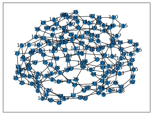
Run the maximum cut (max-cut) problem. The following example demonstrates the Solver's capabilities on a 156-node, 3-regular unweighted graph max-cut problem, but you can also solve weighted graph problems. In addition to qiskit-ibm-catalog, you will also use the following packages to run this example: networkx and numpy. You can install these packages by uncommenting the following cell if you are running this example in a notebook using the IPython kernel.

# %pip install networkx numpy

1. Define the problem

You can run a max-cut problem by defining a graph problem and specifying problem_type='maxcut'.

import networkx as nx
import numpy as np

# Generate a random graph with 156 nodes
maxcut_graph = nx.random_regular_graph(d=3, n=156, seed=8)

# Optionally, visualize the graph
nx.draw_networkx(
    maxcut_graph, nx.kamada_kawai_layout(maxcut_graph), node_size=100
)

The Solver accepts a string as the problem definition input.

# Convert graph to string
problem_as_str = nx.readwrite.json_graph.adjacency_data(maxcut_graph)

2. Run the problem

When using the graph-based input method, specify the problem type.

# This cell is hidden from users
from qiskit_ibm_runtime import QiskitRuntimeService

service = QiskitRuntimeService()
backend_name = service.least_busy(n_qubits=156).name

# Solve the problem
maxcut_job = solver.run(
    problem=problem_as_str,
    problem_type="maxcut",
    backend_name=backend_name,  # E.g. "ibm_fez"
)

Check your Qiskit Function workload's status or return results as follows:

# Print the ID so you can use it later, if necessary
print(maxcut_job.job_id)

# Get job status
print(maxcut_job.status())

34b53970-d95a-4e24-8763-fc6f3d112843

QUEUED

3. Retrieve the result

Retrieve the optimal cut value from the results dictionary.

note

The mapping of the variables to the bitstring may have changed. The output dictionary contains a variables_to_bitstring_index_map sub-dictionary, which helps to verify the ordering.

# Poll for results
maxcut_result = maxcut_job.result()

# Take the absolute value of the solution since the cost function is minimized
qctrl_maxcut = abs(maxcut_result["solution_bitstring_cost"])

# Print the optimal cut value found by the Optimization Solver
print(f"Optimal cut value: {qctrl_maxcut}")

Optimal cut value: 210.0

You can verify the accuracy of the result by solving the problem classically with open-source solvers like PuLP if the graph is not densely connected. High density problems may require advanced classical solvers to validate the solution.

Example: Constrained optimization

The prior max-cut example is a common quadratic unconstrained binary optimization problem. Q-CTRL's Optimization Solver can also solve constrained optimization problems by passing hard constraints directly to the Solver through the constraint input, instead of encoding them as penalty terms in the objective function. The Solver currently supports Hamming-weight-1 constraints: each constraint specifies a group of variables where exactly one variable must equal 1 and the rest must equal 0.

The following example demonstrates how to construct a cost function and a set of hard constraints for a constrained optimization problem, graph partitioning, by assigning every node in a graph to exactly one of several groups while minimizing the total weight of edges whose endpoints land in the same group. In addition to the qiskit-ibm-catalog and qiskit packages, you will also use the following packages to run this example: numpy, networkx, and sympy. You can install these packages by uncommenting the following cell if you are running this example in a notebook using the IPython kernel.

# %pip install numpy networkx sympy

1. Define the problem

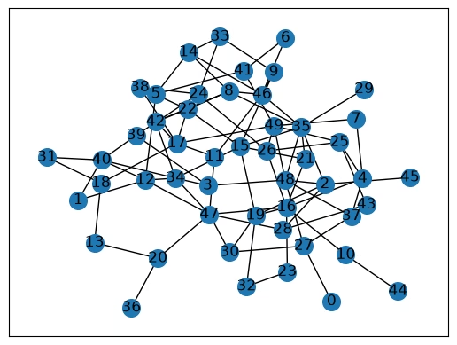
Define a random graph partitioning problem by generating a graph with randomly weighted nodes.

import networkx as nx
from sympy import Symbol, Poly, srepr

# To change the weights, change the seed to any integer.
rng_seed = 18
_rng = np.random.default_rng(rng_seed)
node_count = 50
edge_probability = 0.08
graph = nx.erdos_renyi_graph(
    node_count, edge_probability, seed=rng_seed, directed=False
)

# add node weights
min_weight = -1.0
max_weight = 1.0
for i in graph.nodes:
    weight = (max_weight - min_weight) * _rng.random() + min_weight
    graph.add_node(i, weight=weight)

# Optionally, visualize the graph
nx.draw_networkx(graph, nx.kamada_kawai_layout(graph), node_size=200)

A standard optimization model for weighted graph partitioning can be formulated as follows. Split the nodes of the graph into three groups $g \in \{0, 1, 2\}$, and let $n_{i,g} = 1$ if node $i$ is assigned to group $g$, and $n_{i,g} = 0$ otherwise. The goal is to minimize the total weight of edges whose endpoints are assigned to the same group, where the weight of an edge $(i,j)$ is the combined weight of its two endpoints, $\omega_{i,j} = \omega_i + \omega_j$:

$\textbf{Minimize}\qquad y = \sum_{(i,j)\in E} \omega_{i,j} \sum_{g} n_{i,g}\, n_{j,g}$

# Construct the cost function.
group_count = 3
variables = [
    Symbol(f"n[{i},{g}]")
    for i in range(node_count)
    for g in range(group_count)
]
node_group_var = {
    (i, g): variables[i * group_count + g]
    for i in range(node_count)
    for g in range(group_count)
}
cost_function = Poly(0, *variables)

for i, j in graph.edges():
    edge_weight = graph.nodes[i]["weight"] + graph.nodes[j]["weight"]
    for g in range(group_count):
        cost_function += (
            edge_weight * node_group_var[(i, g)] * node_group_var[(j, g)]
        )

Every node must be assigned to exactly one of the three groups. This is a Hamming-weight-1 constraint: for every node $i$, exactly one of $n_{i,0}, n_{i,1}, n_{i,2}$ must equal 1, and the rest must equal 0:

$n_{i,0} + n_{i,1} + n_{i,2} = 1 \texttt{ for all } i \in V$

Rather than encoding this requirement as a penalty term in the cost function, pass it directly to the Solver as a hard constraint using the constraint input.

# Build the hard constraint: exactly one group per node.
constraint_dict = {
    str(tuple(f"n[{i},{g}]" for g in range(group_count))): 1
    for i in range(node_count)
}
print(f"Problem constraints: {constraint_dict}")

Problem constraints: {"('n[0,0]', 'n[0,1]', 'n[0,2]')": 1, "('n[1,0]', 'n[1,1]', 'n[1,2]')": 1, "('n[2,0]', 'n[2,1]', 'n[2,2]')": 1, "('n[3,0]', 'n[3,1]', 'n[3,2]')": 1, "('n[4,0]', 'n[4,1]', 'n[4,2]')": 1, "('n[5,0]', 'n[5,1]', 'n[5,2]')": 1, "('n[6,0]', 'n[6,1]', 'n[6,2]')": 1, "('n[7,0]', 'n[7,1]', 'n[7,2]')": 1, "('n[8,0]', 'n[8,1]', 'n[8,2]')": 1, "('n[9,0]', 'n[9,1]', 'n[9,2]')": 1, "('n[10,0]', 'n[10,1]', 'n[10,2]')": 1, "('n[11,0]', 'n[11,1]', 'n[11,2]')": 1, "('n[12,0]', 'n[12,1]', 'n[12,2]')": 1, "('n[13,0]', 'n[13,1]', 'n[13,2]')": 1, "('n[14,0]', 'n[14,1]', 'n[14,2]')": 1, "('n[15,0]', 'n[15,1]', 'n[15,2]')": 1, "('n[16,0]', 'n[16,1]', 'n[16,2]')": 1, "('n[17,0]', 'n[17,1]', 'n[17,2]')": 1, "('n[18,0]', 'n[18,1]', 'n[18,2]')": 1, "('n[19,0]', 'n[19,1]', 'n[19,2]')": 1, "('n[20,0]', 'n[20,1]', 'n[20,2]')": 1, "('n[21,0]', 'n[21,1]', 'n[21,2]')": 1, "('n[22,0]', 'n[22,1]', 'n[22,2]')": 1, "('n[23,0]', 'n[23,1]', 'n[23,2]')": 1, "('n[24,0]', 'n[24,1]', 'n[24,2]')": 1, "('n[25,0]', 'n[25,1]', 'n[25,2]')": 1, "('n[26,0]', 'n[26,1]', 'n[26,2]')": 1, "('n[27,0]', 'n[27,1]', 'n[27,2]')": 1, "('n[28,0]', 'n[28,1]', 'n[28,2]')": 1, "('n[29,0]', 'n[29,1]', 'n[29,2]')": 1, "('n[30,0]', 'n[30,1]', 'n[30,2]')": 1, "('n[31,0]', 'n[31,1]', 'n[31,2]')": 1, "('n[32,0]', 'n[32,1]', 'n[32,2]')": 1, "('n[33,0]', 'n[33,1]', 'n[33,2]')": 1, "('n[34,0]', 'n[34,1]', 'n[34,2]')": 1, "('n[35,0]', 'n[35,1]', 'n[35,2]')": 1, "('n[36,0]', 'n[36,1]', 'n[36,2]')": 1, "('n[37,0]', 'n[37,1]', 'n[37,2]')": 1, "('n[38,0]', 'n[38,1]', 'n[38,2]')": 1, "('n[39,0]', 'n[39,1]', 'n[39,2]')": 1, "('n[40,0]', 'n[40,1]', 'n[40,2]')": 1, "('n[41,0]', 'n[41,1]', 'n[41,2]')": 1, "('n[42,0]', 'n[42,1]', 'n[42,2]')": 1, "('n[43,0]', 'n[43,1]', 'n[43,2]')": 1, "('n[44,0]', 'n[44,1]', 'n[44,2]')": 1, "('n[45,0]', 'n[45,1]', 'n[45,2]')": 1, "('n[46,0]', 'n[46,1]', 'n[46,2]')": 1, "('n[47,0]', 'n[47,1]', 'n[47,2]')": 1, "('n[48,0]', 'n[48,1]', 'n[48,2]')": 1, "('n[49,0]', 'n[49,1]', 'n[49,2]')": 1}

Partially constrained problems

You do not need to add every variable to constraint. Any variable left out of the dictionary remains unconstrained, so you can mix hard-constrained groups of variables with free variables in the same problem.

2. Run the problem

# Solve the problem
partition_job = solver.run(
    problem=srepr(cost_function),
    constraint=constraint_dict,
    backend_name="ibm_marrakesh",  # E.g. "ibm_marrakesh"
)

Check your Qiskit Function workload's status or return results as follows:

# Print the ID so you can use it later, if necessary
print(partition_job.job_id)

# Get job status
print(partition_job.status())

b8085944-f313-444e-be39-ea61b1b47ebd
QUEUED

3. Get the result

Retrieve the solution and analyze the results. The solution cost represents the total weight of edges whose endpoints ended up in the same group, so a lower cost indicates a better partitioning of the graph.

partition_result = partition_job.result()
qctrl_cost = partition_result["solution_bitstring_cost"]
solution_bitstring = partition_result["solution_bitstring"]

# Print results
print(f"Total weight of same-group edges: {qctrl_cost}")
print(f"Solution bitstring: {solution_bitstring}")

Total weight of same-group edges: -36.5539
Solution bitstring: 100100100100100001100100100100100100100100100100100001010100010100100100100010001001100100100001100001100001010001001010100100100100100010100100100100

Get support

For any questions or issues, reach out to Q-CTRL.

Changelog

• 2026-08-10: Added support for hard (Hamming weight 1) constraints via the constraint input, and updated the constrained optimization example to use them.
• 2026-02-11: We now have support for ibm_miami

Next steps

Recommendations

• Request access to Q-CTRL Optimization Solver.
• Visit the API reference for this Qiskit Function.
• Try the Solve higher-order binary optimization problems with Q-CTRL's Optimization Solver tutorial.
• Review Sachdeva, N., et al. (2024). Quantum optimization using a 127-qubit gate-model IBM quantum computer can outperform quantum annealers for nontrivial binary optimization problems. arXiv preprint arXiv:2406.01743.
• Review Loco, D., et al. (2026). Practical protein-pocket hydration-site prediction for drug discovery on a quantum computer. arXiv preprint arXiv:2512.08390.
• Review the Mazda case study.
• Review the Network Rail case study.
• Review the Australian Army case study.
• Review the Transport for New South Wales case study.