Approximate quantum compilation for time evolution circuits

Usage estimate: 15 seconds on a Heron processor (NOTE: This is an estimate only. Your runtime might vary.)

Learning outcomes

After completing this tutorial, you can expect to understand the following information:

How to use the AQC-Tensor Qiskit addon to compress deep Trotter circuits into shallow ansatz circuits
How to generate a parametrized ansatz from a Trotter circuit and optimize its parameters using tensor network (MPS) methods
How to evaluate the fidelity of a compressed circuit against the target evolution and run it on quantum hardware

Prerequisites

It is recommended that you familiarize yourself with these topics:

Background

This tutorial demonstrates how to implement Approximate Quantum Compilation using tensor networks (AQC-Tensor) with Qiskit to enhance quantum circuit performance. AQC-Tensor compresses deep Trotter circuits into shallower, more hardware-friendly circuits while preserving simulation accuracy.

How AQC-Tensor works

Consider simulating a Hamiltonian $H$ for total time $t$ using $k$ Trotter steps. The full Trotter circuit is:

U_{\text{full}} = \left[U_{\text{Trotter}}(t/k)\right]^k

A naive approach uses few Trotter steps to keep circuit depth manageable, but this introduces significant Trotter error. AQC-Tensor resolves this tension by separating accuracy from depth:

Target circuit (high accuracy, deep): Construct a Trotter circuit with many steps—say, $10k$ —for the same evolution time. This circuit has far less Trotter error, but is too deep for hardware. Because it is only simulated classically as a matrix product state (MPS), depth is not a concern.
Ansatz circuit (low depth, parametrized): Define a parametrized circuit $V(\theta)$ with the same structure as a single-step Trotter circuit. Initialize it so that $V(\theta_{\text{init}}) = U_{\text{Trotter}}(t/k)$ , then iteratively optimize $\theta$ so that $V(\theta)$ reproduces the high-accuracy target state as closely as possible.

The result is a circuit that retains the depth of a single Trotter step but achieves the accuracy of many, making it feasible for near-term quantum hardware.

When to use AQC-Tensor

AQC-Tensor is most effective when:

Circuit depth exceeds hardware coherence times. If a Trotter simulation requires more Trotter steps than the device can support, AQC-Tensor can compress the evolution into a shallower circuit.
Entanglement remains classically tractable. The total entanglement in a time-evolved state depends primarily on the evolution time $t$ , not the number of Trotter steps $k$ . This means a target circuit with $10k$ steps is typically no harder to represent as an MPS than one with $k$ steps, as long as $t$ is short enough for bond dimensions to stay manageable.
A natural ansatz exists. Because the ansatz mirrors the structure of a Trotter circuit, it provides a physically motivated starting point with well-defined initial parameters, avoiding the convergence issues that can plague arbitrary variational ansatze.

This approach contrasts with generic circuit compression: rather than trying to approximate an arbitrary unitary with fewer gates, AQC-Tensor keeps the same gate structure and optimizes its parameters to reduce Trotter error. See the AQC-Tensor documentation for more information.

This tutorial guides you through the full state-preparation AQC-Tensor workflow: defining a Hamiltonian, generating Trotter circuits, compressing them via tensor-network optimization, and executing the result on IBM Quantum® hardware.

Requirements

Before starting this tutorial, ensure that you have the following installed:

Qiskit SDK v2.0 or later, with visualization support
Qiskit Runtime v0.22 or later (pip install qiskit-ibm-runtime)
AQC-Tensor Qiskit addon (pip install 'qiskit-addon-aqc-tensor[aer,quimb-jax]')

Setup

# Added by doQumentation — required packages for this notebook
!pip install -q matplotlib numpy qiskit qiskit-addon-aqc-tensor qiskit-addon-utils qiskit-ibm-runtime quimb rustworkx scipy

import numpy as np
import quimb.tensor
import datetime
import matplotlib.pyplot as plt

from scipy.linalg import expm
from scipy.optimize import OptimizeResult, minimize

from qiskit.quantum_info import SparsePauliOp, Pauli
from qiskit.transpiler import CouplingMap
from qiskit.transpiler.preset_passmanagers import generate_preset_pass_manager
from qiskit import QuantumCircuit
from qiskit.synthesis import SuzukiTrotter

from qiskit_addon_utils.problem_generators import (
    generate_time_evolution_circuit,
)
from qiskit_addon_aqc_tensor.ansatz_generation import (
    generate_ansatz_from_circuit,
)
from qiskit_addon_aqc_tensor.objective import MaximizeStateFidelity
from qiskit_addon_aqc_tensor.simulation.quimb import QuimbSimulator
from qiskit_addon_aqc_tensor.simulation import tensornetwork_from_circuit
from qiskit_addon_aqc_tensor.simulation import compute_overlap

from qiskit_ibm_runtime import QiskitRuntimeService
from qiskit_ibm_runtime import EstimatorV2 as Estimator
from qiskit_ibm_runtime.fake_provider import FakeKyiv

from rustworkx.visualization import graphviz_draw

Small-scale simulator example

This section uses a 10-site system to illustrate the AQC-Tensor workflow step by step. We simulate the dynamics of a 10-site XXZ spin chain, a widely studied model for examining spin interactions and magnetic properties.

The Hamiltonian is as follows:

\hat{\mathcal{H}}_{XXZ} = \sum_{i=1}^{L-1} J_{i,(i+1)}\left(X_i X_{(i+1)}+Y_i Y_{(i+1)}+ 2\cdot Z_i Z_{(i+1)} \right) \, ,

where $J_{i,(i+1)}$ is a random coefficient for edge $(i, i+1)$ and $L=10$ .

Step 1: Map classical inputs to a quantum problem

In this step, we:

Define the Hamiltonian, observable, and initial state.
Compute the exact expectation value classically for later comparison.
Generate a high-accuracy Trotter circuit (the AQC target) and compress it into a low-depth ansatz using AQC-Tensor.

Set up the Hamiltonian, observable, and initial state

# L is the number of sites in the 1D spin chain
L = 10

# Generate the coupling map
edge_list = [(i - 1, i) for i in range(1, L)]
even_edges = edge_list[::2]
odd_edges = edge_list[1::2]
coupling_map = CouplingMap(edge_list)

# Generate random coefficients for our XXZ Hamiltonian
np.random.seed(0)
Js = np.random.rand(L - 1) + 0.5 * np.ones(L - 1)
hamiltonian = SparsePauliOp(Pauli("I" * L))
for i, edge in enumerate(even_edges + odd_edges):
    hamiltonian += SparsePauliOp.from_sparse_list(
        [
            ("XX", (edge), Js[i] / 2),
            ("YY", (edge), Js[i] / 2),
            ("ZZ", (edge), Js[i]),
        ],
        num_qubits=L,
    )

# Generate a ZZ observable between the two middle qubits
observable = SparsePauliOp.from_sparse_list(
    [("ZZ", (L // 2 - 1, L // 2), 1.0)], num_qubits=L
)

# Generate an initial Néel state |1010101010⟩
initial_state_circuit = QuantumCircuit(L)
for i in range(L):
    if i % 2:
        initial_state_circuit.x(i)

print("Hamiltonian:", hamiltonian)
print("Observable:", observable)
graphviz_draw(coupling_map.graph, method="circo")

Hamiltonian: SparsePauliOp(['IIIIIIIIII', 'IIIIIIIIXX', 'IIIIIIIIYY', 'IIIIIIIIZZ', 'IIIIIIXXII', 'IIIIIIYYII', 'IIIIIIZZII', 'IIIIXXIIII', 'IIIIYYIIII', 'IIIIZZIIII', 'IIXXIIIIII', 'IIYYIIIIII', 'IIZZIIIIII', 'XXIIIIIIII', 'YYIIIIIIII', 'ZZIIIIIIII', 'IIIIIIIXXI', 'IIIIIIIYYI', 'IIIIIIIZZI', 'IIIIIXXIII', 'IIIIIYYIII', 'IIIIIZZIII', 'IIIXXIIIII', 'IIIYYIIIII', 'IIIZZIIIII', 'IXXIIIIIII', 'IYYIIIIIII', 'IZZIIIIIII'],
              coeffs=[1.        +0.j, 0.52440675+0.j, 0.52440675+0.j, 1.0488135 +0.j,
 0.60759468+0.j, 0.60759468+0.j, 1.21518937+0.j, 0.55138169+0.j,
 0.55138169+0.j, 1.10276338+0.j, 0.52244159+0.j, 0.52244159+0.j,
 1.04488318+0.j, 0.4618274 +0.j, 0.4618274 +0.j, 0.9236548 +0.j,
 0.57294706+0.j, 0.57294706+0.j, 1.14589411+0.j, 0.46879361+0.j,
 0.46879361+0.j, 0.93758721+0.j, 0.6958865 +0.j, 0.6958865 +0.j,
 1.391773  +0.j, 0.73183138+0.j, 0.73183138+0.j, 1.46366276+0.j])
Observable: SparsePauliOp(['IIIIZZIIII'],
              coeffs=[1.+0.j])

Output of the previous code cell

Compute the exact expectation value

For a system of this size, we can compute the exact time-evolved expectation value directly using matrix exponentiation. This serves as our ground truth for evaluating the AQC circuit's accuracy.

aqc_evolution_time = 0.2

# Each baseline Trotter step covers dt = aqc_evolution_time / 3
# The subsequent (uncompressed) step covers 1 additional dt
subsequent_evolution_time = aqc_evolution_time / 3
total_evolution_time = aqc_evolution_time + subsequent_evolution_time

# Compute exact expectation value via matrix exponentiation
H_matrix = hamiltonian.to_matrix()
U_exact = expm(-1j * H_matrix * total_evolution_time)

# Build the initial state vector (Néel state)
initial_state_vec = np.zeros(2**L)
state_idx = sum(2**i for i in range(L) if i % 2)
initial_state_vec[state_idx] = 1.0

# Evolve and compute expectation value
evolved_state = U_exact @ initial_state_vec
obs_matrix = observable.to_matrix()
exact_expval = (evolved_state.conj() @ obs_matrix @ evolved_state).real

print(f"AQC evolution time: {aqc_evolution_time}")
print(f"Subsequent evolution time: {subsequent_evolution_time:.6f}")
print(f"Total evolution time: {total_evolution_time:.6f}")
print(f"Exact expectation value: {exact_expval:.6f}")

AQC evolution time: 0.2
Subsequent evolution time: 0.066667
Total evolution time: 0.266667
Exact expectation value: -0.700899

Generate the AQC target circuit

We now construct the Trotter circuit that will serve as the AQC target. This circuit uses many Trotter steps (32) for high accuracy. Because it will only be simulated classically as an MPS—not executed on hardware—the large depth is not a concern.

aqc_target_num_trotter_steps = 32

aqc_target_circuit = initial_state_circuit.copy()
aqc_target_circuit.compose(
    generate_time_evolution_circuit(
        hamiltonian,
        synthesis=SuzukiTrotter(reps=aqc_target_num_trotter_steps),
        time=aqc_evolution_time,
    ),
    inplace=True,
)

Generate an ansatz, initial parameters, subsequent circuit, and a baseline circuit

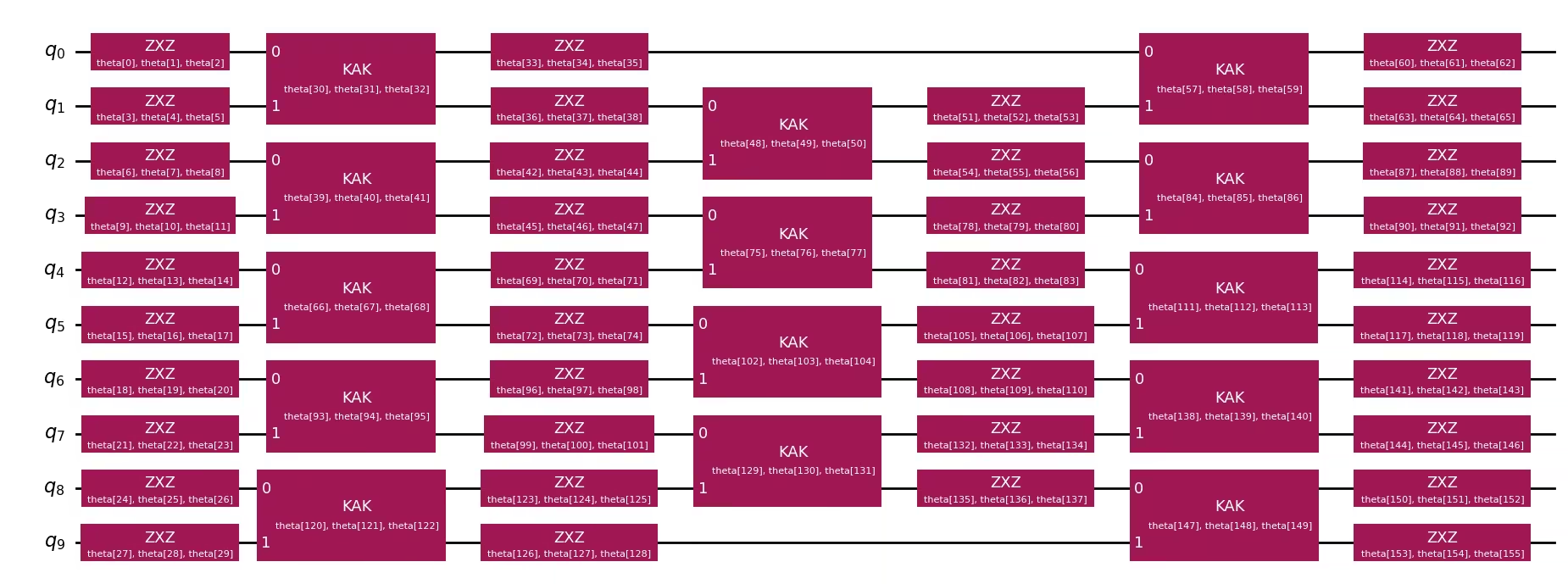
Next, we construct a "good" circuit with the same evolution time as the AQC target but far fewer Trotter steps (only one). We pass this circuit to generate_ansatz_from_circuit, which returns:

A general, parametrized ansatz circuit with the same two-qubit connectivity.
Initial parameters that reproduce the input circuit when plugged into the ansatz.

We also construct:

A subsequent circuit with one Trotter step that will be appended (uncompressed) after the AQC-optimized portion, following the approach in the AQC-Tensor initial state tutorial.
A baseline Trotter circuit using four Trotter steps over the full evolution time (aqc_evolution_time + subsequent_evolution_time). This serves as the comparison: it represents what you would run on hardware without AQC. The AQC ansatz (3 compressed steps + 1 uncompressed step) achieves better accuracy at lower depth.

aqc_ansatz_num_trotter_steps = 1

aqc_good_circuit = initial_state_circuit.copy()
aqc_good_circuit.compose(
    generate_time_evolution_circuit(
        hamiltonian,
        synthesis=SuzukiTrotter(reps=aqc_ansatz_num_trotter_steps),
        time=aqc_evolution_time,
    ),
    inplace=True,
)

aqc_ansatz, aqc_initial_parameters = generate_ansatz_from_circuit(
    aqc_good_circuit
)

# Subsequent circuit: 1 non-compressed Trotter step appended after AQC
subsequent_num_trotter_steps = 1
subsequent_circuit = generate_time_evolution_circuit(
    hamiltonian,
    synthesis=SuzukiTrotter(reps=subsequent_num_trotter_steps),
    time=subsequent_evolution_time,
)

# Baseline Trotter circuit: 4 Trotter steps over total evolution time, no AQC
baseline_num_trotter_steps = 4
baseline_circuit = initial_state_circuit.copy()
baseline_circuit.compose(
    generate_time_evolution_circuit(
        hamiltonian,
        synthesis=SuzukiTrotter(reps=baseline_num_trotter_steps),
        time=total_evolution_time,
    ),
    inplace=True,
)

print(
    f"Target circuit:      depth {aqc_target_circuit.depth(lambda x: x.operation.num_qubits == 2)}"
)
print(
    f"Baseline circuit:    depth {baseline_circuit.depth(lambda x: x.operation.num_qubits == 2)} ({baseline_num_trotter_steps} Trotter steps, time={total_evolution_time:.4f})"
)
print(
    f"Subsequent circuit:  depth {subsequent_circuit.depth(lambda x: x.operation.num_qubits == 2)} ({subsequent_num_trotter_steps} Trotter step, time={subsequent_evolution_time:.4f})"
)
print(
    f"Ansatz circuit:      depth {aqc_ansatz.depth(lambda x: x.operation.num_qubits == 2)}, with {len(aqc_initial_parameters)} parameters"
)
aqc_ansatz.draw("mpl", fold=-1)

Target circuit:      depth 384
Baseline circuit:    depth 48 (4 Trotter steps, time=0.2667)
Subsequent circuit:  depth 12 (1 Trotter step, time=0.0667)
Ansatz circuit:      depth 3, with 156 parameters

Output of the previous code cell

Set up tensor network simulation and build the target MPS

We use the quimb matrix-product state (MPS) circuit simulator, with JAX providing automatic differentiation for the gradient-based optimization. We then build an MPS representation of the target state and evaluate the starting fidelity between the initial ansatz and the target. As the problem instance is a relatively small example, the starting fidelity starts off quite high.

simulator_settings = QuimbSimulator(
    quimb.tensor.CircuitMPS, autodiff_backend="jax"
)

aqc_target_mps = tensornetwork_from_circuit(
    aqc_target_circuit, simulator_settings
)
print("Target MPS maximum bond dimension:", aqc_target_mps.psi.max_bond())

good_mps = tensornetwork_from_circuit(aqc_good_circuit, simulator_settings)
starting_fidelity = abs(compute_overlap(good_mps, aqc_target_mps)) ** 2
print(f"Starting fidelity: {starting_fidelity:.6f}")

Target MPS maximum bond dimension: 5
Starting fidelity: 0.998246

Optimize the ansatz parameters

We minimize the MaximizeStateFidelity cost function using the L-BFGS-B optimizer. The optimizer iteratively adjusts the ansatz parameters to maximize the fidelity between the ansatz circuit and the target MPS.

aqc_stopping_fidelity = 1
aqc_max_iterations = 500

stopping_point = 1.0 - aqc_stopping_fidelity
objective = MaximizeStateFidelity(
    aqc_target_mps, aqc_ansatz, simulator_settings
)

def callback(intermediate_result: OptimizeResult):
    fidelity = 1 - intermediate_result.fun
    print(
        f"{datetime.datetime.now()} Intermediate result: Fidelity {fidelity:.8f}"
    )
    if intermediate_result.fun < stopping_point:
        raise StopIteration

result = minimize(
    objective,
    aqc_initial_parameters,
    method="L-BFGS-B",
    jac=True,
    options={"maxiter": aqc_max_iterations},
    callback=callback,
)
if result.status not in (0, 1, 99):
    raise RuntimeError(
        f"Optimization failed: {result.message} (status={result.status})"
    )

print(f"Done after {result.nit} iterations.")
aqc_final_parameters = result.x

2026-05-18 13:14:49.731596 Intermediate result: Fidelity 0.99952882
2026-05-18 13:14:49.734425 Intermediate result: Fidelity 0.99958531
2026-05-18 13:14:49.737101 Intermediate result: Fidelity 0.99960093
2026-05-18 13:14:49.739813 Intermediate result: Fidelity 0.99961046
2026-05-18 13:14:49.742969 Intermediate result: Fidelity 0.99962560
2026-05-18 13:14:49.745916 Intermediate result: Fidelity 0.99964395
2026-05-18 13:14:49.748615 Intermediate result: Fidelity 0.99968150
2026-05-18 13:14:49.753684 Intermediate result: Fidelity 0.99970569
2026-05-18 13:14:49.756208 Intermediate result: Fidelity 0.99973788
2026-05-18 13:14:49.759067 Intermediate result: Fidelity 0.99975385
2026-05-18 13:14:49.762321 Intermediate result: Fidelity 0.99976458
2026-05-18 13:14:49.765526 Intermediate result: Fidelity 0.99977661
2026-05-18 13:14:49.768496 Intermediate result: Fidelity 0.99978663
2026-05-18 13:14:49.771278 Intermediate result: Fidelity 0.99980236
2026-05-18 13:14:49.773735 Intermediate result: Fidelity 0.99981607
2026-05-18 13:14:49.776339 Intermediate result: Fidelity 0.99982811
2026-05-18 13:14:49.779177 Intermediate result: Fidelity 0.99985827
2026-05-18 13:14:49.782243 Intermediate result: Fidelity 0.99988354
2026-05-18 13:14:49.784904 Intermediate result: Fidelity 0.99991608
2026-05-18 13:14:49.787737 Intermediate result: Fidelity 0.99993336
2026-05-18 13:14:49.790414 Intermediate result: Fidelity 0.99993956
2026-05-18 13:14:49.793029 Intermediate result: Fidelity 0.99994421
2026-05-18 13:14:49.795585 Intermediate result: Fidelity 0.99994743
2026-05-18 13:14:49.835045 Intermediate result: Fidelity 0.99994791
2026-05-18 13:14:49.839786 Intermediate result: Fidelity 0.99994803
2026-05-18 13:14:49.842403 Intermediate result: Fidelity 0.99994898
2026-05-18 13:14:49.873779 Intermediate result: Fidelity 0.99994898
Done after 27 iterations.

Assemble the final AQC circuit

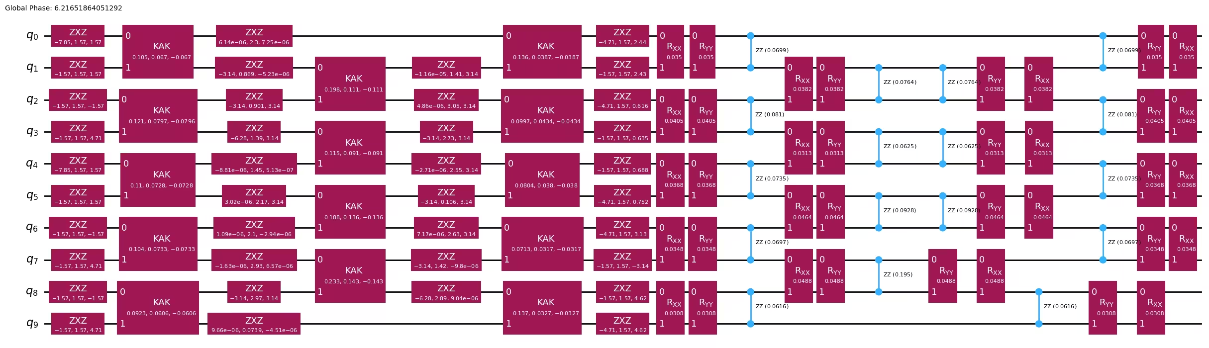
With the optimized parameters in hand, we bind them to the ansatz and then append the subsequent (uncompressed) Trotter step. The resulting circuit has the depth of a single compressed Trotter step plus one uncompressed step, but the compressed portion approximates the accuracy of 32 Trotter steps.

aqc_final_circuit = aqc_ansatz.assign_parameters(aqc_final_parameters)
aqc_final_circuit.compose(subsequent_circuit, inplace=True)
aqc_final_circuit.draw("mpl", fold=-1)

Output of the previous code cell

Step 2: Optimize problem for quantum hardware execution

For this small-scale example, we use a fake backend (FakeKyiv) to simulate hardware execution locally. We transpile both the AQC-optimized circuit (aqc_final_circuit) and the baseline Trotter circuit (baseline_circuit, four Trotter steps over the full evolution time, no AQC) to the backend's instruction set architecture (ISA), with optimization_level=3 to further reduce circuit depth.

backend = FakeKyiv()

pass_manager = generate_preset_pass_manager(
    backend=backend, optimization_level=3
)

# Transpile the AQC-optimized circuit (compressed + subsequent step)
isa_circuit = pass_manager.run(aqc_final_circuit)
isa_observable = observable.apply_layout(isa_circuit.layout)
print(
    "AQC circuit depth:",
    isa_circuit.depth(lambda x: x.operation.num_qubits == 2),
)

# Transpile the baseline Trotter circuit (no AQC optimization)
isa_baseline_circuit = pass_manager.run(baseline_circuit)
isa_baseline_observable = observable.apply_layout(isa_baseline_circuit.layout)
print(
    "Baseline Trotter circuit depth:",
    isa_baseline_circuit.depth(lambda x: x.operation.num_qubits == 2),
)

AQC circuit depth: 15
Baseline Trotter circuit depth: 27

Step 3: Execute using Qiskit primitives

We use the EstimatorV2 primitive with the fake backend to run both the AQC-optimized circuit and the baseline Trotter circuit, measuring the ZZ observable for each.

estimator = Estimator(backend)

# Run both circuits
aqc_result = estimator.run([(isa_circuit, isa_observable)]).result()
baseline_result = estimator.run(
    [(isa_baseline_circuit, isa_baseline_observable)]
).result()

Step 4: Post-process and return result in desired classical format

We extract the expectation values from both runs and compare them to the exact result. The baseline Trotter circuit shows what we would get without AQC at the same circuit depth, while the AQC circuit demonstrates the improvement from tensor-network optimization.

aqc_expval = aqc_result[0].data.evs.tolist()
baseline_expval = baseline_result[0].data.evs.tolist()

print(f"Exact:              {exact_expval:.4f}")
print(
    f"Baseline Trotter:   {baseline_expval:.4f}, |\u0394| = {np.abs(exact_expval - baseline_expval):.4f}  (depth {isa_baseline_circuit.depth(lambda x: x.operation.num_qubits == 2)}, {baseline_num_trotter_steps} steps)"
)
print(
    f"AQC (3+1):          {aqc_expval:.4f}, |\u0394| = {np.abs(exact_expval - aqc_expval):.4f}  (depth {isa_circuit.depth(lambda x: x.operation.num_qubits == 2)}, compressed+subsequent)"
)

Exact:              -0.7009
Baseline Trotter:   -0.5400, |Δ| = 0.1609  (depth 27, 4 steps)
AQC (3+1):          -0.5728, |Δ| = 0.1281  (depth 15, compressed+subsequent)

plt.style.use("seaborn-v0_8")

labels = [
    f"Baseline Trotter\n({baseline_num_trotter_steps} steps, depth {isa_baseline_circuit.depth(lambda x: x.operation.num_qubits == 2)})",
    f"AQC (3+1)\n(depth {isa_circuit.depth(lambda x: x.operation.num_qubits == 2)})",
]
values = [baseline_expval, aqc_expval]
colors = ["tab:orange", "tab:blue"]

plt.figure(figsize=(8, 5))
bars = plt.bar(labels, values, color=colors, width=0.5)
plt.axhline(
    y=exact_expval,
    color="tab:green",
    linestyle="--",
    linewidth=2,
    label=f"Exact ({exact_expval:.4f})",
)
plt.ylabel("Expected Value")
plt.title(
    "AQC-Tensor (3 compressed + 1 uncompressed) vs Baseline Trotter (10-site XXZ)"
)
plt.legend()
for bar in bars:
    y_val = bar.get_height()
    plt.text(
        bar.get_x() + bar.get_width() / 2.0,
        y_val,
        f"{y_val:.4f}",
        ha="center",
        va="bottom" if y_val >= 0 else "top",
    )
plt.axhline(y=0, color="black", linewidth=0.3)
plt.tight_layout()
plt.show()

Output of the previous code cell

Large-scale hardware example

We now scale up to a 50-site XXZ model to demonstrate AQC-Tensor on a more realistic problem size. The workflow is the same as the small-scale example: we compress three Trotter steps via AQC and append one uncompressed step.

For a system of this size, matrix exponentiation is infeasible ( $2^{50}$ dimensions), so we compute the reference expectation value directly from a high-accuracy MPS evolved for the full time.

Steps 1–4 combined

# -------------------------Step 1-------------------------

# Define the 50-site spin chain
L = 50
edge_list = [(i - 1, i) for i in range(1, L)]
even_edges = edge_list[::2]
odd_edges = edge_list[1::2]
coupling_map = CouplingMap(edge_list)

# Random XXZ Hamiltonian
np.random.seed(0)
Js = np.random.rand(L - 1) + 0.5 * np.ones(L - 1)
hamiltonian = SparsePauliOp(Pauli("I" * L))
for i, edge in enumerate(even_edges + odd_edges):
    hamiltonian += SparsePauliOp.from_sparse_list(
        [
            ("XX", (edge), Js[i] / 2),
            ("YY", (edge), Js[i] / 2),
            ("ZZ", (edge), Js[i]),
        ],
        num_qubits=L,
    )

observable = SparsePauliOp.from_sparse_list(
    [("ZZ", (L // 2 - 1, L // 2), 1.0)], num_qubits=L
)

# Initial Néel state
initial_state_circuit = QuantumCircuit(L)
for i in range(L):
    if i % 2:
        initial_state_circuit.x(i)

# Time parameters
aqc_evolution_time = 0.2
subsequent_evolution_time = aqc_evolution_time / 3
total_evolution_time = aqc_evolution_time + subsequent_evolution_time

# AQC target circuit (high-accuracy, 32 Trotter steps for AQC portion)
aqc_target_num_trotter_steps = 32

aqc_target_circuit = initial_state_circuit.copy()
aqc_target_circuit.compose(
    generate_time_evolution_circuit(
        hamiltonian,
        synthesis=SuzukiTrotter(reps=aqc_target_num_trotter_steps),
        time=aqc_evolution_time,
    ),
    inplace=True,
)

# Generate ansatz from 1-step Trotter circuit
aqc_good_circuit = initial_state_circuit.copy()
aqc_good_circuit.compose(
    generate_time_evolution_circuit(
        hamiltonian,
        synthesis=SuzukiTrotter(reps=1),
        time=aqc_evolution_time,
    ),
    inplace=True,
)

aqc_ansatz, aqc_initial_parameters = generate_ansatz_from_circuit(
    aqc_good_circuit
)

# Subsequent circuit: 1 non-compressed Trotter step
subsequent_circuit = generate_time_evolution_circuit(
    hamiltonian,
    synthesis=SuzukiTrotter(reps=1),
    time=subsequent_evolution_time,
)

# Baseline Trotter circuit: 4 Trotter steps over total evolution time, no AQC
baseline_num_trotter_steps = 4
baseline_circuit = initial_state_circuit.copy()
baseline_circuit.compose(
    generate_time_evolution_circuit(
        hamiltonian,
        synthesis=SuzukiTrotter(reps=baseline_num_trotter_steps),
        time=total_evolution_time,
    ),
    inplace=True,
)
print(
    f"Target circuit:  depth {aqc_target_circuit.depth(lambda x: x.operation.num_qubits == 2)}"
)
print(
    f"Ansatz circuit:  depth {aqc_ansatz.depth(lambda x: x.operation.num_qubits == 2)}, with {len(aqc_initial_parameters)} parameters"
)
print(
    f"Subsequent circuit: depth {subsequent_circuit.depth(lambda x: x.operation.num_qubits == 2)}"
)
print(
    f"Baseline circuit:   depth {baseline_circuit.depth(lambda x: x.operation.num_qubits == 2)} ({baseline_num_trotter_steps} steps, time={total_evolution_time:.4f})"
)

# Build target MPS and compute reference expectation value
simulator_settings = QuimbSimulator(
    quimb.tensor.CircuitMPS, autodiff_backend="jax"
)
aqc_target_mps = tensornetwork_from_circuit(
    aqc_target_circuit, simulator_settings
)
print("Target MPS maximum bond dimension:", aqc_target_mps.psi.max_bond())

# For the reference expectation value, we need the full evolution (AQC + subsequent)
# Build a high-accuracy full circuit for MPS reference
full_target_circuit = initial_state_circuit.copy()
full_target_circuit.compose(
    generate_time_evolution_circuit(
        hamiltonian,
        synthesis=SuzukiTrotter(reps=aqc_target_num_trotter_steps),
        time=total_evolution_time,
    ),
    inplace=True,
)
full_target_mps = tensornetwork_from_circuit(
    full_target_circuit, simulator_settings
)
exact_expval = full_target_mps.local_expectation(
    quimb.pauli("Z") & quimb.pauli("Z"), (L // 2 - 1, L // 2)
).real.item()
print(f"Reference expectation value (from MPS): {exact_expval:.6f}")

# Optimize ansatz parameters
objective = MaximizeStateFidelity(
    aqc_target_mps, aqc_ansatz, simulator_settings
)

def callback(intermediate_result: OptimizeResult):
    fidelity = 1 - intermediate_result.fun
    print(
        f"{datetime.datetime.now()} Intermediate result: Fidelity {fidelity:.8f}"
    )

result = minimize(
    objective,
    aqc_initial_parameters,
    method="L-BFGS-B",
    jac=True,
    options={"maxiter": 500},
    callback=callback,
)
if result.status not in (0, 1, 99):
    raise RuntimeError(
        f"Optimization failed: {result.message} (status={result.status})"
    )
print(f"Done after {result.nit} iterations.")

# Assemble the final AQC circuit: optimized ansatz + subsequent Trotter step
aqc_final_circuit = aqc_ansatz.assign_parameters(result.x)
aqc_final_circuit.compose(subsequent_circuit, inplace=True)

# -------------------------Step 2-------------------------

service = QiskitRuntimeService()
backend = service.least_busy(min_num_qubits=127)
print(backend)

pass_manager = generate_preset_pass_manager(
    backend=backend, optimization_level=3
)
isa_circuit = pass_manager.run(aqc_final_circuit)
isa_observable = observable.apply_layout(isa_circuit.layout)
print(
    "AQC circuit depth:",
    isa_circuit.depth(lambda x: x.operation.num_qubits == 2),
)

# Also transpile the baseline Trotter circuit (4 Trotter steps, no AQC)
isa_baseline_circuit = pass_manager.run(baseline_circuit)
isa_baseline_observable = observable.apply_layout(isa_baseline_circuit.layout)
print(
    "Baseline Trotter circuit depth:",
    isa_baseline_circuit.depth(lambda x: x.operation.num_qubits == 2),
)

# -------------------------Step 3-------------------------

# Submit both circuits in a single job
estimator = Estimator(backend)
estimator.options.environment.job_tags = ["TUT_AQCTE"]

job = estimator.run(
    [
        (isa_circuit, isa_observable),
        (isa_baseline_circuit, isa_baseline_observable),
    ]
)
print("Job ID:", job.job_id())

Target circuit:  depth 385
Ansatz circuit:  depth 7, with 816 parameters
Subsequent circuit: depth 12
Baseline circuit:   depth 49 (4 steps, time=0.2667)
Target MPS maximum bond dimension: 5
Reference expectation value (from MPS): -0.738669
2026-05-18 13:02:11.219150 Intermediate result: Fidelity 0.99795732
2026-05-18 13:02:11.232256 Intermediate result: Fidelity 0.99822481
2026-05-18 13:02:11.245160 Intermediate result: Fidelity 0.99829520
2026-05-18 13:02:11.257765 Intermediate result: Fidelity 0.99832379
2026-05-18 13:02:11.270280 Intermediate result: Fidelity 0.99836416
2026-05-18 13:02:11.284116 Intermediate result: Fidelity 0.99840073
2026-05-18 13:02:11.296856 Intermediate result: Fidelity 0.99846863
2026-05-18 13:02:11.309602 Intermediate result: Fidelity 0.99865244
2026-05-18 13:02:11.322012 Intermediate result: Fidelity 0.99872665
2026-05-18 13:02:11.334195 Intermediate result: Fidelity 0.99892335
2026-05-18 13:02:11.346570 Intermediate result: Fidelity 0.99901045
2026-05-18 13:02:11.359202 Intermediate result: Fidelity 0.99907181
2026-05-18 13:02:11.371511 Intermediate result: Fidelity 0.99911125
2026-05-18 13:02:11.383870 Intermediate result: Fidelity 0.99918585
2026-05-18 13:02:11.396184 Intermediate result: Fidelity 0.99921504
2026-05-18 13:02:11.408543 Intermediate result: Fidelity 0.99924936
2026-05-18 13:02:11.422557 Intermediate result: Fidelity 0.99929226
2026-05-18 13:02:11.436275 Intermediate result: Fidelity 0.99933099
2026-05-18 13:02:11.449511 Intermediate result: Fidelity 0.99935792
2026-05-18 13:02:11.462093 Intermediate result: Fidelity 0.99937925
2026-05-18 13:02:11.475783 Intermediate result: Fidelity 0.99940690
2026-05-18 13:02:11.490254 Intermediate result: Fidelity 0.99944409
2026-05-18 13:02:11.503292 Intermediate result: Fidelity 0.99946840
2026-05-18 13:02:11.516064 Intermediate result: Fidelity 0.99949378
2026-05-18 13:02:11.532861 Intermediate result: Fidelity 0.99951380
2026-05-18 13:02:11.546182 Intermediate result: Fidelity 0.99955313
2026-05-18 13:02:11.559168 Intermediate result: Fidelity 0.99955707
2026-05-18 13:02:11.571753 Intermediate result: Fidelity 0.99959306
2026-05-18 13:02:11.584257 Intermediate result: Fidelity 0.99960486
2026-05-18 13:02:11.597610 Intermediate result: Fidelity 0.99961714
2026-05-18 13:02:11.610106 Intermediate result: Fidelity 0.99962953
2026-05-18 13:02:11.622515 Intermediate result: Fidelity 0.99963525
2026-05-18 13:02:11.635543 Intermediate result: Fidelity 0.99964658
2026-05-18 13:02:11.649044 Intermediate result: Fidelity 0.99965027
2026-05-18 13:02:11.664148 Intermediate result: Fidelity 0.99965802
2026-05-18 13:02:11.678033 Intermediate result: Fidelity 0.99966731
2026-05-18 13:02:11.692714 Intermediate result: Fidelity 0.99967780
2026-05-18 13:02:11.706753 Intermediate result: Fidelity 0.99968567
2026-05-18 13:02:11.720780 Intermediate result: Fidelity 0.99969139
2026-05-18 13:02:11.733471 Intermediate result: Fidelity 0.99969628
2026-05-18 13:02:11.745998 Intermediate result: Fidelity 0.99970331
2026-05-18 13:02:11.758424 Intermediate result: Fidelity 0.99970796
2026-05-18 13:02:11.771986 Intermediate result: Fidelity 0.99971165
2026-05-18 13:02:11.785841 Intermediate result: Fidelity 0.99971892
2026-05-18 13:02:11.799105 Intermediate result: Fidelity 0.99972226
2026-05-18 13:02:11.811623 Intermediate result: Fidelity 0.99972441
2026-05-18 13:02:11.824114 Intermediate result: Fidelity 0.99972679
2026-05-18 13:02:11.837179 Intermediate result: Fidelity 0.99972965
2026-05-18 13:02:12.345479 Intermediate result: Fidelity 0.99972965
Done after 49 iterations.
<IBMBackend('ibm_pittsburgh')>
AQC circuit depth: 71
Baseline Trotter circuit depth: 111
Job ID: d85kc6o0bvlc73d5nhn0

# -------------------------Step 4-------------------------

hw_results = job.result()
aqc_expval = hw_results[0].data.evs.tolist()
baseline_expval = hw_results[1].data.evs.tolist()

print(f"Exact (MPS):        {exact_expval:.4f}")
print(
    f"Baseline Trotter:   {baseline_expval:.4f}, |\u0394| = {np.abs(exact_expval - baseline_expval):.4f}"
)
print(
    f"AQC (3+1):          {aqc_expval:.4f}, |\u0394| = {np.abs(exact_expval - aqc_expval):.4f}"
)

labels = [
    f"Baseline Trotter\n({baseline_num_trotter_steps} steps, depth {isa_baseline_circuit.depth(lambda x: x.operation.num_qubits == 2)})",
    f"AQC (3+1)\n(depth {isa_circuit.depth(lambda x: x.operation.num_qubits == 2)})",
]
values = [baseline_expval, aqc_expval]
colors = ["tab:orange", "tab:blue"]

plt.figure(figsize=(8, 5))
bars = plt.bar(labels, values, color=colors, width=0.5)
plt.axhline(
    y=exact_expval,
    color="tab:green",
    linestyle="--",
    linewidth=2,
    label=f"Exact ({exact_expval:.4f})",
)
plt.ylabel("Expected Value")
plt.title(
    "AQC-Tensor (3 compressed + 1 uncompressed) vs Baseline Trotter (50-site XXZ)"
)
plt.legend()
for bar in bars:
    y_val = bar.get_height()
    plt.text(
        bar.get_x() + bar.get_width() / 2.0,
        y_val,
        f"{y_val:.4f}",
        ha="center",
        va="bottom" if y_val >= 0 else "top",
    )
plt.axhline(y=0, color="black", linewidth=0.3)
plt.tight_layout()
plt.show()

Exact (MPS):        -0.7387
Baseline Trotter:   -0.5955, |Δ| = 0.1432
AQC (3+1):          -0.6734, |Δ| = 0.0653

Output of the previous code cell

Next steps

Recommendations

If you found this work interesting, you might be interested in the following material:

AQC-Tensor addon documentation — includes the related unitary AQC technique, which optimizes parametrized circuits to approximate a target unitary operator rather than a prepared state
Error mitigation and suppression techniques
Combine error mitigation techniques

Learning outcomes​

Prerequisites​

Background​

How AQC-Tensor works​

When to use AQC-Tensor​

Requirements​

Setup​

Small-scale simulator example​

Step 1: Map classical inputs to a quantum problem​

Set up the Hamiltonian, observable, and initial state​

Compute the exact expectation value​

Generate the AQC target circuit​

Generate an ansatz, initial parameters, subsequent circuit, and a baseline circuit​

Set up tensor network simulation and build the target MPS​

Optimize the ansatz parameters​

Assemble the final AQC circuit​

Step 2: Optimize problem for quantum hardware execution​

Step 3: Execute using Qiskit primitives​

Step 4: Post-process and return result in desired classical format​

Large-scale hardware example​

Steps 1–4 combined​

Next steps​

Learning outcomes

Prerequisites

Background

How AQC-Tensor works

When to use AQC-Tensor

Requirements

Setup

Small-scale simulator example

Step 1: Map classical inputs to a quantum problem

Set up the Hamiltonian, observable, and initial state

Compute the exact expectation value

Generate the AQC target circuit

Generate an ansatz, initial parameters, subsequent circuit, and a baseline circuit

Set up tensor network simulation and build the target MPS

Optimize the ansatz parameters

Assemble the final AQC circuit

Step 2: Optimize problem for quantum hardware execution

Step 3: Execute using Qiskit primitives

Step 4: Post-process and return result in desired classical format

Large-scale hardware example

Steps 1–4 combined

Next steps