Nuclear magnetic resonance with Qiskit

For this Qiskit in Classrooms module, students must have a working Python environment with the following packages installed:

• qiskit v2.1 or newer
• qiskit-ibm-runtime v0.40.1 or newer
• qiskit-aer v0.17 or newer
• scipy and matplotlib (for fitting and plotting)
• pylatexenc (for rendering circuit diagrams)

To set up and install the packages above, see the Install Qiskit guide. To run jobs on real quantum computers, students must set up an account with IBM Quantum® by following the steps in the Set up your IBM Cloud® account guide.

This module has been tested and uses approximately 5 minutes of QPU time. This is an estimate, and your actual usage might vary.

Introduction

When a chemist runs an NMR experiment, they place a sample of nuclear spins in a strong magnetic field, apply a radio-frequency (RF) pulse, and measure the signal that comes back. The technique rests on a few ideas from the quantum mechanics of a spin-1/2 particle in a magnetic field. The spin has two energy levels separated by an energy that corresponds to a characteristic Larmor frequency. A resonant pulse at that frequency tips the spin into the transverse plane, where it precesses and induces a signal that then fades with two characteristic times, $T_1$ and $T_2$.

A superconducting qubit is an engineered version of the same object: a controllable two-level quantum system. Its $|0\rangle$ and $|1\rangle$ states are the analog of spin-up and spin-down, the gate we apply to rotate it is the analog of the RF pulse, and it loses coherence with its own $T_1$ and $T_2$. This is not merely a loose comparison; some of the earliest experimental quantum processors in the late 1990s and early 2000s used NMR.

In this module you will use a real quantum computer to run the same characterization experiments that an NMR spectroscopist (or a quantum engineer calibrating hardware) performs:

• Rabi / nutation — driving the spin and watching it rotate. This is how you calibrate a $\pi$ or $\pi/2$ rotation.
• $T_1$ — spin-lattice relaxation, the decay of an excited spin back to equilibrium.
• $T_2$ — spin-spin relaxation (dephasing), measured with a Ramsey experiment and refocused with a Hahn echo.
• NMR spectroscopy (chemical shift and $J$-coupling) — simulating a small molecule on several qubits and reading its multiplet spectrum to recover connectivity through the $n+1$ rule.

For each concept we first give the minimal theory, then implement the experiment in Qiskit following the four-step Qiskit patterns workflow.

Theory

Spin-1/2 particles in a magnetic field

A spin-1/2 nucleus has a magnetic moment $\boldsymbol{\mu} = \gamma \hbar \mathbf{I}$, where $\gamma$ is the gyromagnetic ratio. In a static field $B_0$ along $z$, the two spin states split in energy (the Zeeman effect):

$E_{\pm} = \mp \tfrac{1}{2}\gamma \hbar B_0, \qquad \Delta E = \gamma \hbar B_0 = \hbar \omega_0 .$

The energy gap defines the Larmor (resonance) frequency $\omega_0 = \gamma B_0$. The magnetic moment precesses about $B_0$ at this same frequency.

To rotate the spin we apply an oscillating RF field at (or near) $\omega_0$. In the frame rotating at the drive frequency (the rotating frame), a resonant drive rotates the Bloch vector about an axis in the $x$-$y$ plane. How far it rotates (the flip angle) is set by the pulse's strength and duration. Two choices matter most: a $90^\circ$ pulse tips a $+1/2$ spin into the transverse plane, and a $180^\circ$ pulse rotates it fully to $-1/2$.

Translating between NMR and quantum computing jargon

A qubit is a two-level system, mathematically identical to a spin-1/2 in a magnetic field — so while we're running on a quantum processor rather than a nucleus, the physics is the same physics that underlies NMR. Only the vocabulary differs. This table helps you talk to physical chemists and quantum-computing specialists alike.

NMR / spin-1/2	Quantum processor (qubit)
Spin-up / spin-down	$\ket{0}$ / $\ket{1}$
Zeeman gap $\Delta E = \hbar\omega_0$	Qubit transition energy $\hbar\omega_{01}$
Larmor frequency $\omega_0$	Qubit frequency $\omega_{01}$
Resonant RF pulse (flip angle $\theta$)	Single-qubit rotation gate $R_X(\theta)$
$90^\circ$ / $180^\circ$ pulse	$R_X(\pi/2)$ / $R_X(\pi)$
Spin-lattice relaxation $T_1$	Qubit energy-relaxation time $T_1$
Spin-spin relaxation $T_2$	Qubit dephasing time $T_2$
Nutation	Rabi oscillations
Free induction decay (FID), Hahn echo	Ramsey, echo sequences

Everything below is an exercise in measuring the right-hand column and reading it as the left-hand column.

Set up the Qiskit environment

We follow the Qiskit patterns workflow throughout:

1. Map the problem to a quantum circuit.
2. Optimize the circuit for execution (transpile to the backend).
3. Execute using an IBM Quantum primitive.
4. Post-process and analyze.

First we load the runtime service and pick the least-busy real backend. If you haven't yet saved your credentials, see the documentation page on how to save your login credentials.

# Added by doQumentation — installs the packages this notebook needs if they are missing
import importlib.util

_needed = {"matplotlib": "matplotlib", "numpy": "numpy", "qiskit": "qiskit", "qiskit_aer": "qiskit-aer", "qiskit_ibm_runtime": "qiskit-ibm-runtime", "scipy": "scipy"}
_missing = [pip for module, pip in _needed.items()
            if importlib.util.find_spec(module) is None]
# One at a time, so a package that fails to install does not block the others
for _pip in _missing:
    %pip install -q {_pip}
if not _missing:
    print("\u2713 All required packages are installed")

# Load the IBM Quantum Compute Service and select the least-busy real backend
from qiskit_ibm_runtime import QiskitRuntimeService, SamplerV2 as Sampler, Batch

# After setup, this picks up your saved credentials automatically:
service = QiskitRuntimeService()

backend = service.least_busy(operational=True, simulator=False, min_num_qubits=156)
print(f"Selected backend: {backend.name}")

Selected backend: ibm_kingston

Use the cell below to switch between real hardware and a local simulator for the whole notebook. Running on hardware is the point of the module, but if there are connectivity or usage issues, the simulator can be a backup. Set USE_HARDWARE = True to run on the QPU selected above.

import numpy as np
from itertools import combinations
from qiskit_aer import AerSimulator
from qiskit.transpiler import generate_preset_pass_manager
from qiskit_ibm_runtime import EstimatorV2 as Estimator

USE_HARDWARE = True  # <-- set True to run on the QPU selected above
USE_BATCH = False  # Safer for a class with pauses; set True for an uninterrupted run

if USE_HARDWARE:
    run_backend = backend  # the real QPU selected above
else:
    # Local testing mode: an Aer simulator that mimics the selected device -- its noise model,
    # coupling map, and qubit count -- while layout choices still use real calibration data.
    run_backend = AerSimulator.from_backend(backend)

# --- Choose connected qubits with low readout error. --------------------------------------
def readout_error(q):
    props = backend.target["measure"].get((q,))
    return props.error if props is not None and props.error is not None else 1.0

coupling_map = backend.coupling_map or backend.target.build_coupling_map()
edges = {tuple(sorted(edge)) for edge in coupling_map.get_edges() if edge[0] != edge[1]}

# AX needs one connected pair.
AX_LAYOUT = list(min(edges, key=lambda edge: sum(readout_error(q) for q in edge)))

# AX2 needs one qubit connected to two neighbours; the first entry is the central A qubit.
neighbors = {q: set() for q in range(backend.num_qubits)}
for q0, q1 in edges:
    neighbors[q0].add(q1)
    neighbors[q1].add(q0)
ax2_layouts = (
    [a, x1, x2]
    for a, adjacent in neighbors.items()
    for x1, x2 in combinations(adjacent, 2)
)
AX2_LAYOUT = min(ax2_layouts, key=lambda layout: sum(readout_error(q) for q in layout))

# Use a long-lived qubit for the single-qubit experiments.
def best_qubit(backend):
    return max(
        range(backend.num_qubits), key=lambda q: backend.qubit_properties(q).t2 or 0.0
    )

QUBIT = best_qubit(backend)
qp = backend.qubit_properties(QUBIT)
print(
    f"Using qubit {QUBIT} for single-qubit experiments: "
    f"T1 = {qp.t1 * 1e6:.0f} us, T2 = {qp.t2 * 1e6:.0f} us"
)
print(f"Using physical qubits {AX_LAYOUT} for AX")
print(f"Using physical qubits {AX2_LAYOUT} for AX2 (A first, then the two X spins)")

pm_q = generate_preset_pass_manager(
    optimization_level=1, backend=run_backend, initial_layout=[QUBIT]
)
pm_ax = generate_preset_pass_manager(
    optimization_level=1, backend=run_backend, initial_layout=AX_LAYOUT
)
pm_ax2 = generate_preset_pass_manager(
    optimization_level=1, backend=run_backend, initial_layout=AX2_LAYOUT
)

# Job mode is the default because a classroom pause can deactivate a Batch. On the Open plan,
# a Batch has a 10-minute maximum lifetime and deactivates after 1 minute with no queued job.
batch = Batch(backend=run_backend) if USE_BATCH else None
execution_mode = batch if batch is not None else run_backend
sampler = Sampler(mode=execution_mode)
estimator = Estimator(mode=execution_mode)
estimator.options.resilience_level = 0  # raw expectation values, no error mitigation
estimator.options.default_shots = 1000

mode_name = "Batch" if USE_BATCH else "individual jobs"
device_name = "hardware" if USE_HARDWARE else "local simulator (runtime local mode)"
print(f"Ready. Running on {device_name} using {mode_name}.")

Experiment: Rabi oscillations (nutation)

Theory

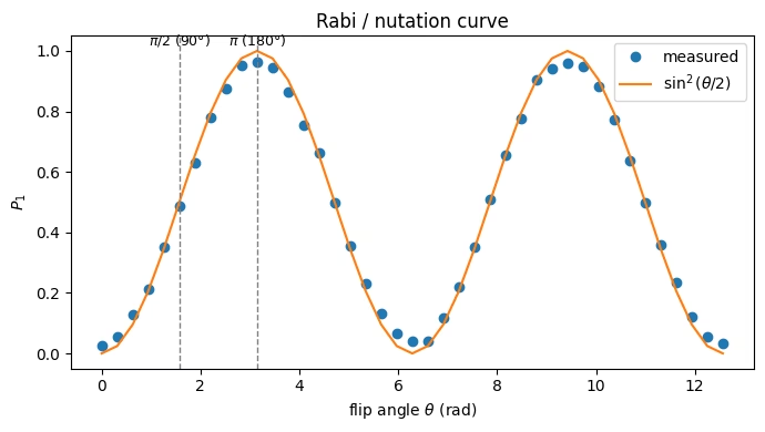
Drive a spin on resonance and its Bloch vector rotates steadily from pole to pole — it nutates. If we apply a rotation of flip angle $\theta$ about the $x$-axis to a qubit starting in $|0\rangle$, the probability of finding it in $|1\rangle$ is:

$P_1(\theta) = \sin^2\!\left(\tfrac{\theta}{2}\right) = \tfrac{1}{2}\bigl(1 - \cos\theta\bigr).$

This is the Rabi curve. Its first maximum is the $\pi$ pulse (full inversion, the $180^\circ$ pulse); a $\pi/2$ pulse is a quarter-turn (the $90^\circ$ pulse that tips a spin into the transverse plane). In NMR this curve is how you calibrate your pulses.

Experimental caveat

A literal Rabi experiment sweeps the drive amplitude or duration in time. That requires pulse-level control, which was removed in Qiskit v2.0. Here we instead sweep the rotation angle $\theta$ of an $R_X(\theta)$ gate. The curve and the $\pi$/$\pi/2$ identification are identical; the only difference is that we choose an angle directly instead of calibrating a pulse length. On hardware with fractional gates, $R_X(\theta)$ for arbitrary $\theta$ runs natively.

A Bloch-sphere view

The animation below shows the nutation: a resonant drive rotates the Bloch vector steadily about the $x$-axis, carrying it from $|0\rangle$ down toward $|1\rangle$ and back. This is the very motion the Rabi curve measures.

Map the problem to a circuit

We build one parameterized circuit, $R_X(\theta)$ followed by a measurement, and later evaluate it at many angles at once.

from qiskit import QuantumCircuit
from qiskit.circuit import Parameter

theta = Parameter("theta")
rabi = QuantumCircuit(1, 1)
rabi.rx(theta, 0)
rabi.measure(0, 0)
rabi.draw("mpl")

Optimize for execution

Transpile to an Instruction Set Architecture (ISA) circuit for the chosen backend.

rabi_isa = pm_q.run(rabi)

Execute

We sweep $\theta$ from $0$ to $4\pi$ (two full Rabi cycles). Passing an array of parameter values as a single Primitive Unified Bloc (PUB) runs them all in one job.

angles = np.linspace(0, 4 * np.pi, 41)
job = sampler.run([(rabi_isa, angles.reshape(-1, 1))], shots=1000)
rabi_result = job.result()

Post-process and analyze

Extract $P_1$ at each angle and compare to $\sin^2(\theta/2)$.

import matplotlib.pyplot as plt

ba = rabi_result[0].data.c  # BitArray, one entry per angle
shots = ba.num_shots
p1 = np.array([ba.get_counts(i).get("1", 0) / shots for i in range(len(angles))])

plt.figure(figsize=(7, 4))
plt.plot(angles, p1, "o", label="measured")
plt.plot(angles, np.sin(angles / 2) ** 2, "-", label=r"$\sin^2(\theta/2)$")
for k, name in [(np.pi / 2, r"$\pi/2$ (90°)"), (np.pi, r"$\pi$ (180°)")]:
    plt.axvline(k, color="gray", ls="--", lw=1)
    plt.text(k, 1.02, name, ha="center", fontsize=9)
plt.xlabel(r"flip angle $\theta$ (rad)")
plt.ylabel(r"$P_1$")
plt.title("Rabi / nutation curve")
plt.legend()
plt.tight_layout()
plt.show()

Check your understanding

On the curve you measured, $P_1$ first reaches its maximum at the $\pi$ pulse ($\theta = \pi$). Now suppose a device is miscalibrated, so that a nominal angle $\theta$ on the x-axis actually produces a rotation of $1.05\,\theta$.

(a) At what nominal angle would the first maximum of $P_1$ now appear? (b) Would applying a single $\pi$ pulse be a sensitive way to detect this 5% error?

Answer

(a) The maximum appears where the actual rotation equals $\pi$, that is, at the nominal angle $\theta = \pi/1.05 \approx 0.95\pi$ — a small leftward shift of the peak.

(b) No. A nominal $\pi$ pulse produces an actual rotation of $1.05\pi$, giving $P_1 = \sin^2(1.05\pi/2) \approx 0.994$ instead of $1$ — a change too small to see against measurement noise. This is why, to calibrate precisely, NMR spectroscopists amplify the error by applying the rotation many times (for example the $360^\circ$ method, or a long pulse train), so a small per-pulse error accumulates into a large, measurable deviation. We return to this idea in the challenge problems.

Experiment: $T_1$ (spin-lattice relaxation)

Theory

Left alone, an excited spin gives up energy to its surroundings (the "lattice") and relaxes back toward thermal equilibrium. The excited-state population decays exponentially with the spin-lattice relaxation time $T_1$:

$P_1(\tau) = e^{-\tau/T_1}.$

For a chemist, $T_1$ sets the recycle delay you must wait between scans for quantitative NMR, and it reports on molecular tumbling and dynamics. On a qubit it is the energy-relaxation time, and is one of the two main numbers used to model the decoherence effects in a quantum computer.

The experiment. Prepare $|1\rangle$ with an $X$ gate (a $\pi$ pulse), wait a variable delay $\tau$, then measure. The fraction still in $|1\rangle$ traces out the decay.

A Bloch-sphere view

$T_1$ relaxation returns the excited state to equilibrium, so the Bloch vector slides from $|1\rangle$ back up to $|0\rangle$ along the $z$-axis.

Build and transpile a delay scan

Delay durations must be concrete values (they are scheduled in hardware time), so we build one circuit per delay.

# Scale the T1 delay sweep to the qubit's reported coherence, and snap each delay to an integer
# number of samples (dt) so there are no "duration rounded" warnings (as in the Ramsey/echo cells).
T1_us = (backend.qubit_properties(QUBIT).t1 or 100e-6) * 1e6  # reported T1 (us)
delays_us = np.linspace(0, 5 * T1_us, 20)  # 0 .. ~5 T1 captures the full decay
print(f"T1 sweep: 0..{5*T1_us:.0f} us in {len(delays_us)} points")

dt = backend.dt
t1_circuits = []
for tau in delays_us:
    n_dt = int(round(tau * 1e-6 / dt))  # integer samples -> no rounding warning
    qc = QuantumCircuit(1, 1)
    qc.x(0)  # pi pulse: prepare |1>
    qc.delay(n_dt, 0, unit="dt")  # wait tau
    qc.measure(0, 0)
    t1_circuits.append(qc)

t1_isa = pm_q.run(t1_circuits)

T1 sweep: 0..1393 us in 20 points

Execute

t1_job = sampler.run([(c,) for c in t1_isa], shots=1000)
t1_res = t1_job.result()

Analyze — fit the exponential

from scipy.optimize import curve_fit

p1_t1 = np.array(
    [r.data.c.get_counts().get("1", 0) / r.data.c.num_shots for r in t1_res]
)

def decay(t, A, T1, B):
    return A * np.exp(-t / T1) + B

p0 = [1.0, 100.0, 0.0]
popt, _ = curve_fit(decay, delays_us, p1_t1, p0=p0, maxfev=10000)
T1_fit = popt[1]

plt.figure(figsize=(7, 4))
plt.plot(delays_us, p1_t1, "o", label="measured")
tt = np.linspace(0, delays_us.max(), 200)
plt.plot(tt, decay(tt, *popt), "-", label=rf"fit: $T_1$ = {T1_fit:.1f} µs")
plt.xlabel("delay τ (µs)")
plt.ylabel(r"$P_1$")
plt.title("$T_1$ relaxation")
plt.legend()
plt.tight_layout()
plt.show()
print(f"Measured T1 = {T1_fit:.1f} microseconds")

Measured T1 = 225.3 microseconds

The exact $T_1$ time varies from experiment to experiment and backend to backend, but you should see a result of around a few hundred microseconds.

Check your understanding

In quantitative NMR you are told to wait about $5\,T_1$ between scans. Using the decay law, what fraction of the equilibrium magnetization has recovered after $5\,T_1$?

Answer

After $5\,T_1$, the remaining deviation from equilibrium is $e^{-5}\approx 0.0067$, that is, about 99.3% recovered.

Experiment: $T_2$, $T_2^*$

Theory

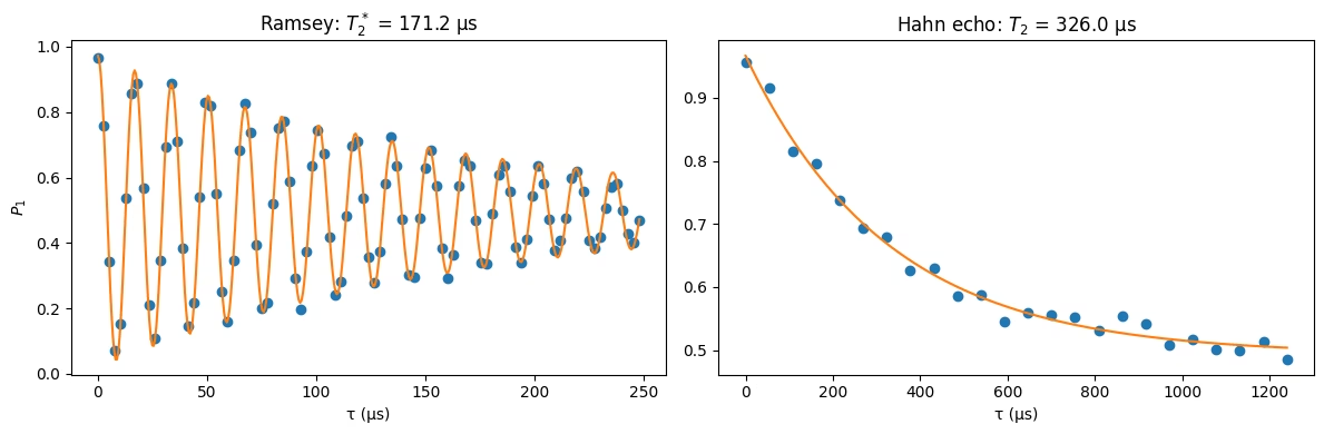
$T_1$ measures energy loss. $T_2$ measures loss of phase coherence in the transverse plane. We can observe this with a Ramsey experiment: a $\pi/2$ pulse rotates all the spins down to the equator, all pointing in the same direction. They Larmor precess, but each one precesses at a slightly different frequency, so they fan out along the equator and the net transverse signal decays, with a characteristic decay time of $T_2^*$.

Aside for quantum readers: The fanning-out picture shows one way to lose coherence: a spread of definite phases that average out. It's worth knowing this isn't the only mechanism. Coherence can also be lost because the phase becomes entangled with the environment, so it's no longer a definite value the system holds at all. You can't tell the two mechanisms apart just by watching the signal decay, so the fanning-out picture is a good intuition. Be mindful not to read it as the complete or literal story.

Two effects dephase a spin:

• Irreversible (or effectively irreversible) decoherence arising from uncontrolled coupling to other degrees of freedom, characterized by the true $T_2$. In NMR, this generally comes from molecular motion modulating the couplings between spins. In quantum computing, it corresponds to unwanted couplings between qubits and the environment.
• Static or slowly-varying, reversible frequency offsets, such as field inhomogeneity, qubit-to-qubit frequency variation, and calibration errors. Combined with the true $T_2$, these produce the shorter apparent decay time $T_2^*$ observed in a Ramsey experiment.

So how do we recover the true $T_2$ if a Ramsey experiment only tells us about $T_2^*$? The second experiment, called a Hahn echo, cancels all the noise of the second type to find the true $T_2$. It starts the same as a Ramsey experiment, with a $\pi/2$ pulse, then the spins fan out as before. After some time $\tau$, a $\pi$ pulse is applied. The pulse reverses the phase accumulation caused by static frequency offsets, so the spins refocus after a second delay of the same duration, $\tau$.

$T_2^*$ and $T_2$ are both important numbers to know in both the chemistry setting and the quantum computing setting. In the chemistry setting, $T_2^*$ sets your linewidth for a standard NMR experiment (you'll see what this means in a later section). $T_2$ can tell you much about the molecules, such as molecular tumbling, and a change in $T_2$ can signal that a molecule has bound to something larger. In the quantum computing setting, we generally want both $T_2$ and $T_2^*$ to be as long as possible, so we have more time to perform experiments before decoherence overwhelms the system. A whole family of techniques based on the Hahn echo extends this time by canceling the reversible noise, so that the circuit is ideally limited by the true $T_2$, not $T_2^*$. This is called "dynamical decoupling."

Implementation

When we implement the Ramsey and Hahn echo experiments on a qubit, the readout is slightly different than for the NMR case. In NMR, you can directly observe the oscillating fields induced by the spins precessing at the Larmor frequency in the transverse plane. But with a qubit, we can only measure its projection along the $Z$ axis, that is, whether it's $\vert 0 \rangle$ or $\vert 1 \rangle$. Therefore, for both experiments, we end with an additional $\pi/2$ pulse followed by a measurement. This $\pi/2$ pulse translates the phase information of the qubit into a population.

Below we run each experiment to determine $T_2^*$ and $T_2$.

Ramsey ($T_2^{*}$): Two $\pi/2$ pulses with delay time $\tau$

The first $\pi/2$ pulse tips the Bloch vector to the equator, and the next one translates the phase of the Bloch vector to a population. Because the phase changes in time as the Bloch vector precesses, we see a sinusoidal pattern in the population as a function of precession time $\tau$. As the qubit loses phase coherence we should see the amplitude of this sine curve decay.

Some more subtleties for the quantum readers: In quantum computing experiments, the oscillations we see aren't actually at the Larmor frequency, which is in the GHz range and much too fast for us to resolve. Quantum experiments operate in the rotating frame: a frame that spins along with the qubit at (near) the Larmor frequency, so the fast precession is invisible and the Bloch vector looks nearly still. To see fringes, we deliberately set our rotating frame slightly detuned from the Larmor frequency. The Bloch vector then appears to precess at that small detuning, and we get an oscillating signal at the detuning frequency. Below, we don't fix the detuning at one value; we choose it so that about a dozen fringes span the measurement window (which we size to the qubit's coherence time), which keeps the oscillation easy to sample without aliasing. One more wrinkle: in Qiskit we don't have the pulse-level control needed to change the pulse frequency (which is what sets the rotating-frame frequency). Instead, we add an effective detuning by hand, using it to set the phase of the second Ramsey pulse. It's a bit contrived, but the result is the same and the decay we observe is still the genuine $T_2^*$.

A Bloch-sphere view

A $\pi/2$ pulse tips the spins to the equator; each then precesses at a slightly different rate and they fan out, so the net (red) vector shrinks as they dephase — this decay is $T_2^*$.

# Adaptive Ramsey: scale the window to the reported coherence and choose the detuning so a fixed
# number of fringes span it. This decouples the point count from the window -- a long window stays
# cheap and cannot alias (we keep 8 samples per fringe).
T2_us = (backend.qubit_properties(QUBIT).t2 or 100e-6) * 1e6  # reported (echo) T2 (us)
ramsey_span = 0.5 * T2_us  # window = half the reported T2
n_fringes = 12  # fringes across the window
f_detune = n_fringes / (
    ramsey_span * 1e-6
)  # adaptive detuning (Hz) -> low, so a long window is cheap
samp_per_fringe = 8
n_ramsey = n_fringes * samp_per_fringe + 1  # ~97 points, fixed regardless of T2
ramsey_delays_us = np.linspace(0, ramsey_span, n_ramsey)
print(
    f"Ramsey sweep: 0..{ramsey_span:.0f} us in {n_ramsey} points "
    f"(detuning {f_detune/1e3:.1f} kHz, {samp_per_fringe} samples/fringe)"
)

dt = backend.dt  # seconds per sample
delays_dt = [int(round(t * 1e-6 / dt)) for t in ramsey_delays_us]  # integer samples
actual_delays_us = np.array(delays_dt) * dt * 1e6  # true (snapped) delays for fitting

ramsey_circ = []
for n_dt, tau_us in zip(delays_dt, actual_delays_us):
    qc = QuantumCircuit(1, 1)
    qc.rx(np.pi / 2, 0)
    qc.delay(n_dt, 0, unit="dt")  # integer duration -> no rounding warning
    qc.rz(
        2 * np.pi * f_detune * tau_us * 1e-6, 0
    )  # detuning phase (uses the true delay)
    qc.rx(np.pi / 2, 0)
    qc.measure(0, 0)
    ramsey_circ.append(qc)

ramsey_isa = pm_q.run(ramsey_circ)
ramsey_res = sampler.run([(c,) for c in ramsey_isa], shots=1000).result()
p1_ramsey = np.array(
    [r.data.c.get_counts().get("1", 0) / r.data.c.num_shots for r in ramsey_res]
)

ramsey_circ[len(ramsey_circ) // 2].draw("mpl")  # draw a sample circuit (mid-sweep)

Ramsey sweep: 0..248 us in 97 points (detuning 48.4 kHz, 8 samples/fringe)

Hahn echo ($T_2$): Add a refocusing $\pi$ pulse in the middle

A Bloch-sphere view

The Hahn echo: the spins fan out as before, then a $\pi$ pulse flips them, so their continued precession refocuses them back together (the red vector regrows), recovering the coherence lost to static dephasing.

# Scale the echo sweep to the reported (echo) T2. The echo signal is monotonic (no fringes),
# so only the range matters here; 0 .. ~2.5 T2 shows the full decay for a clean fit.
T2_us = (backend.qubit_properties(QUBIT).t2 or 100e-6) * 1e6
echo_delays_us = np.linspace(0, 2.5 * T2_us, 24)  # total free-evolution time
print(f"Echo sweep: 0..{2.5*T2_us:.0f} us in {len(echo_delays_us)} points")

dt = backend.dt
half_dt = [
    int(round(t / 2 * 1e-6 / dt)) for t in echo_delays_us
]  # samples per half-delay
actual_echo_us = np.array(half_dt) * 2 * dt * 1e6  # true total delay for fitting

echo_circ = []
for n_half in half_dt:
    qc = QuantumCircuit(1, 1)
    qc.rx(np.pi / 2, 0)
    qc.delay(n_half, 0, unit="dt")  # half the free-evolution, integer samples
    qc.rx(np.pi, 0)  # refocusing pi pulse
    qc.delay(n_half, 0, unit="dt")
    qc.rx(-np.pi / 2, 0)
    qc.measure(0, 0)
    echo_circ.append(qc)

echo_isa = pm_q.run(echo_circ)
echo_res = sampler.run([(c,) for c in echo_isa], shots=1000).result()
p1_echo = np.array(
    [r.data.c.get_counts().get("1", 0) / r.data.c.num_shots for r in echo_res]
)

echo_circ[len(echo_circ) // 2].draw("mpl")  # draw a sample circuit

Echo sweep: 0..1240 us in 24 points

Analyze: Fit and compare the two decays

# Initial guesses / bounds derived from the reported coherence so the fits track the scaled axes.
T2_us = (backend.qubit_properties(QUBIT).t2 or 100e-6) * 1e6

# Ramsey: decaying oscillation -> extract T2*
def ramsey_fn(t, A, T2s, f, phi, B):
    return A * np.exp(-t / T2s) * np.cos(2 * np.pi * f * t + phi) + B

rp0 = [0.4, T2_us / 2, f_detune * 1e-6, 0.0, 0.5]  # T2* guess ~ half the echo T2
rbounds = (
    [0, 0.1, 0, -np.pi, 0],
    [1, 2 * T2_us, 5, np.pi, 1],
)  # keep the fit from collapsing to ~0
rpopt, _ = curve_fit(
    ramsey_fn, ramsey_delays_us, p1_ramsey, p0=rp0, bounds=rbounds, maxfev=20000
)
T2_star = abs(rpopt[1])

# Echo: simple exponential envelope -> extract T2
def env(t, A, T2, B):
    return A * np.exp(-t / T2) + B

epopt, _ = curve_fit(env, echo_delays_us, p1_echo, p0=[0.5, T2_us, 0.0], maxfev=10000)
T2 = abs(epopt[1])

fig, ax = plt.subplots(1, 2, figsize=(12, 4))
ax[0].plot(ramsey_delays_us, p1_ramsey, "o")
tt = np.linspace(0, ramsey_delays_us.max(), 400)
ax[0].plot(tt, ramsey_fn(tt, *rpopt), "-")
ax[0].set_title(rf"Ramsey: $T_2^*$ = {T2_star:.1f} µs")
ax[0].set_xlabel("τ (µs)")
ax[0].set_ylabel(r"$P_1$")
ax[1].plot(echo_delays_us, p1_echo, "o")
tt2 = np.linspace(0, echo_delays_us.max(), 400)
ax[1].plot(tt2, env(tt2, *epopt), "-")
ax[1].set_title(rf"Hahn echo: $T_2$ = {T2:.1f} µs")
ax[1].set_xlabel("τ (µs)")
plt.tight_layout()
plt.show()
print(f"T2* (Ramsey) = {T2_star:.1f} µs ;  T2 (echo) = {T2:.1f} µs")

T2* (Ramsey) = 171.2 µs ;  T2 (echo) = 326.0 µs

Here we see both the Ramsey oscillation and the Hahn echo signal decay, as expected. The associated time scales for each of these decays are $T_2^*$ and $T_2$, respectively.

Check your understanding

You should typically find $T_2 \gtrsim T_2^{*}$. Explain why in one sentence, and say what physical effect the Hahn echo's $\pi$ pulse removes, as well as what it cannot remove.

Answer

$T_2^{*}$ includes both irreversible dephasing and reversible static spread, so it decays faster; the echo's $\pi$ pulse refocuses the static, reversible dephasing (field inhomogeneity / fixed-frequency offsets), leaving only the irreversible spin-spin dephasing, which is the true $T_2$. The echo cannot undo fluctuations that change between the two halves of the sequence.

NMR spectroscopy of a molecule: Chemical shift and $J$-coupling

From one spin to a molecule

The experiments so far characterized a single, isolated spin. Real chemical NMR reads a molecule (many coupled spins at once) and uses the resulting spectrum to infer features of the molecule's structure. This can tell us about two effects:

• Chemical shift. Each chemically distinct nucleus precesses at a slightly different frequency $\nu_i$, because its local electrons shield the applied field by different amounts. Peak positions therefore identify chemical environments (a CH$_3$ proton versus an aromatic one, for example).
• Scalar $J$-coupling. A through-bond interaction between two spins splits each peak into a multiplet. A nucleus with $n$ equivalent neighbors is split into $n+1$ lines with binomial intensities, the $n+1$ rule. The splitting pattern reveals connectivity (which nuclei are bonded), and the spacing is the coupling constant $J$.

The experiment

To model this in our quantum computer, we need to implement a spin Hamiltonian on the qubits. In the weak-coupling, high-field limit (chemical-shift differences $\gg$ couplings), the $XX$ and $YY$ parts of the coupling average out, leaving only $ZZ$. So the Hamiltonian is (angular-frequency units, $\hbar=1$):

$H = \underbrace{\sum_i \pi\,\nu_i\, Z_i}_{\text{chemical shift}} \;+\; \underbrace{\sum_{i<j} \tfrac{\pi}{2}\,J_{ij}\, Z_iZ_j}_{J\text{-coupling}}.$

Each nucleus is one qubit: the chemical shift is a single-qubit $Z$ rotation, and the coupling is a two-qubit $ZZ$ interaction.

The experiment proceeds as follows. A $\pi/2$ pulse tips every spin into the transverse plane, and the spins precess and couple for time $t$. We record the complex transverse magnetization $s(t) = \langle X\rangle + i\langle Y\rangle$ summed over all spins. As in the Ramsey experiment above, this transverse magnetization traces out a decaying sinusoid as a function of the precession time $t$. When we take the Fourier transform of the signal, we get a spectrum with peaks at the chemical shift $\nu_i$ split by the scalar coupling $J_{ij}$.

note

We simulate the molecule's evolution by mapping the time $t$ onto rotation angles: a larger $t$ means larger $Z$ and $ZZ$ rotations, not a longer or deeper circuit. So while the simulated state does advance with $t$ (that's what makes the free induction decay (FID) oscillate), the physical qubits never idle any longer and there's no $t$-dependent decoherence. The simulated FID therefore never decays on its own. For an infinitely long ideal FID the spectral lines would be infinitely sharp; our finite sampling window instead gives them finite resolution and can introduce spectral leakage. Real NMR lines have a finite width set by $T_2^*$. We add it back by multiplying the FID by a window $e^{-t/T_2^{*}}$ before the Fourier transform. This is called a line-broadening apodization, which spectroscopists apply in processing to set the linewidth (trading resolution for signal-to-noise). (An optional cell in the Appendix of this module shows a Trotterized alternative, where the decay instead comes from real decoherence that grows with circuit depth.)

The AX system

Let's start with the so-called AX system, a molecule consisting of two coupled, chemically distinct spins. The labels A and X denote the two chemically distinct spin environments. The letters are arbitrary, but the fact that they are far apart in the alphabet illustrates their chemical dissimilarity.

Map and optimize

We write one function that, given the chemical-shift offsets $\nu_i$ and couplings $J_{ij}$, returns a parameterized state-preparation circuit. The $\pi/2$ pulse tips the spins to the equator, then the $Z$ rotations simulate the evolution of the state under the chemical-shift and $J$-coupling terms. Each $\nu_i$ is a small precession offset in Hz relative to a chosen reference, or rotating-frame carrier. Here we set it manually; in a real molecule, electron shielding changes the local magnetic field and shifts each nucleus's resonance relative to that reference. This is modeled by the single-qubit $R_Z$ gates, one per spin, and each $\nu_i$ fixes where that spin's peak sits in the spectrum. The two-qubit $ZZ$ gate applies the coupling $J_{ij}$, which splits each peak into a multiplet and sets the spacing between its lines.

from qiskit import QuantumCircuit
from qiskit.circuit import Parameter
from qiskit.quantum_info import SparsePauliOp

t = Parameter(
    "t"
)  # evolution time (arbitrary units; the frequencies below are in matching units)

def fid_circuit(offsets, couplings):
    """State-preparation circuit for a set of spins: a pi/2 pulse, then evolution under the
    chemical-shift + J-coupling Hamiltonian for time t. No measurement -- the Estimator reads
    <X> and <Y> directly.

    offsets   : list of chemical-shift frequencies nu_i, one per qubit
    couplings : dict {(i, j): J_ij}
    """
    n = len(offsets)
    qc = QuantumCircuit(n)
    qc.ry(np.pi / 2, range(n))  # pi/2 pulse: tip every spin into the transverse plane
    for i, nu in enumerate(offsets):
        qc.rz(2 * np.pi * nu * t, i)  # chemical-shift precession -> line at nu_i
    for (i, j), J in couplings.items():
        qc.rzz(np.pi * J * t, i, j)  # J-coupling -> splitting of size J
    return qc

def transverse_obs(n):
    """Total transverse observables (sum over spins): (sum_i X_i, sum_i Y_i)."""
    ox = SparsePauliOp.from_sparse_list(
        [("X", [i], 1.0) for i in range(n)], num_qubits=n
    )
    oy = SparsePauliOp.from_sparse_list(
        [("Y", [i], 1.0) for i in range(n)], num_qubits=n
    )
    return ox, oy

# AX system: two distinct chemical shifts, one coupling
ax_offsets = [6.0, -6.0]  # chemical shifts nu_1, nu_2 (Hz)
ax_couplings = {(0, 1): 2.0}  # J_12 = 2 Hz

ax_isa = pm_ax.run(fid_circuit(ax_offsets, ax_couplings))
fid_circuit(ax_offsets, ax_couplings).draw("mpl")

Execute and post-process

We evaluate the circuit over a grid of evolution times, and the Estimator returns $\langle X\rangle$ and $\langle Y\rangle$ at each. We combine these into the complex FID $\langle X\rangle + i\langle Y\rangle$, apply the apodization window, and Fourier transform the result to obtain the spectrum.

# --- time grid ---
n_t = 128  # number of FID samples
dt = 1 / 32  # time step -> Nyquist frequency = 1/(2 dt) = 16 Hz
times = np.arange(n_t) * dt

# --- Step 3-4: Estimator returns <X> and <Y> directly (both quadratures in one job) ---
def run_fid(isa_circ, n, est):
    """Complex FID s(t) = sum_i <X_i> + i <Y_i> over the time grid, via the Estimator."""
    ox, oy = transverse_obs(n)
    ox = ox.apply_layout(isa_circ.layout)  # map observables onto the transpiled qubits
    oy = oy.apply_layout(isa_circ.layout)
    params = times.reshape(-1, 1)
    res = est.run(
        [(isa_circ, ox, params), (isa_circ, oy, params)]
    ).result()  # both quadratures, one job
    return res[0].data.evs + 1j * res[1].data.evs

def spectrum(fid, T2=1.0):
    sig = fid * np.exp(-times / T2)  # apodization -> Lorentzian linewidth ~ 1/(pi T2)
    spec = np.fft.fftshift(np.fft.fft(sig))
    freq = np.fft.fftshift(np.fft.fftfreq(len(times), dt))
    return freq, np.abs(spec)

fid_ax = run_fid(ax_isa, n=2, est=estimator)
freq, spec = spectrum(fid_ax, T2=1.0)

fig, ax = plt.subplots(1, 2, figsize=(12, 4))
ax[0].plot(times, fid_ax.real, label=r"Re $s(t)=\langle X\rangle$")
ax[0].plot(times, fid_ax.imag, label=r"Im $s(t)=\langle Y\rangle$")
ax[0].set_xlabel("evolution time $t$")
ax[0].set_ylabel("transverse signal")
ax[0].set_title("AX free induction decay")
ax[0].legend()
ax[1].plot(freq, spec)
for nu in ax_offsets:
    for s in (-1, 1):
        ax[1].axvline(nu + s * ax_couplings[(0, 1)] / 2, color="gray", ls="--", lw=1)
ax[1].set_xlim(-12, 12)
ax[1].set_xlabel(r"frequency $\nu$ (Hz)")
ax[1].set_ylabel("intensity")
ax[1].set_title("AX spectrum: two doublets, split by $J$")
plt.tight_layout()
plt.show()
print(
    "Expected AX lines (Hz):",
    sorted({nu + s * ax_couplings[(0, 1)] / 2 for nu in ax_offsets for s in (-1, 1)}),
)

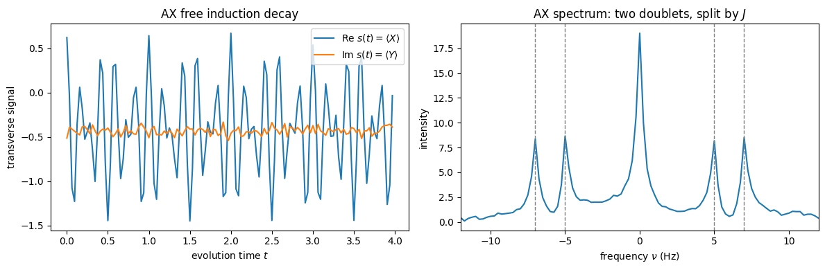
Expected AX lines (Hz): [-7.0, -5.0, 5.0, 7.0]

Extension: An AX$_2$ system and the $n+1$ rule

Now add a second equivalent neighbor. In an AX$_2$ system one A spin couples, with the same $J$, to two equivalent X spins. (Remember, X is just a label for the two equivalent spins; it has nothing to do with the Pauli $X$ operators. Every coupling below is still $ZZ$.) Spin A then sees four neighbor configurations $(\uparrow\uparrow,\ \uparrow\downarrow,\ \downarrow\uparrow,\ \downarrow\downarrow)$; the two mixed ones coincide, so A is split into a 1:2:1 triplet ($n=2 \Rightarrow n+1 = 3$ lines). Each X spin sees only A and stays a doublet. Equivalent spins do not split each other, so we include no X–X coupling.

A real molecule with this pattern is 1,1,2-trichloroethane (Cl$_2$CH–CH$_2$Cl). When targeting the hydrogen spins (which is the most common form of NMR), the single hydrogen proton in CH plays the role of A, and the two equivalent CH$_2$ protons are the two X spins. Now just count neighbors: the CH proton has two neighbors (the CH$_2$ pair), so its signal splits into a 1:2:1 triplet ($n=2$); each CH$_2$ proton has only one neighbor (the CH), so the CH$_2$ signal is a 1:1 doublet ($n=1$). Note that the group with fewer protons (CH) shows more lines; the line count reflects how many neighbors a signal has, not how many protons share it.

Below, we simulate an AX$_2$ system with three qubits.

# AX2: spin A (qubit 0) coupled equally to two equivalent X spins (qubits 1, 2)
ax2_offsets = [6.0, -6.0, -6.0]  # A at +6 Hz; the two X both at -6 Hz
ax2_couplings = {
    (0, 1): 2.0,
    (0, 2): 2.0,
}  # equal A-X couplings; no coupling between the X spins

ax2_isa = pm_ax2.run(fid_circuit(ax2_offsets, ax2_couplings))
fid_ax2 = run_fid(ax2_isa, n=3, est=estimator)
freq2, spec2 = spectrum(fid_ax2, T2=1.0)

fig, ax = plt.subplots(1, 2, figsize=(12, 4))
ax[0].plot(times, fid_ax2.real, label=r"Re $s(t)=\langle X\rangle$")
ax[0].plot(times, fid_ax2.imag, label=r"Im $s(t)=\langle Y\rangle$")
ax[0].set_xlabel("evolution time $t$")
ax[0].set_ylabel("transverse signal")
ax[0].set_title("AX$_2$ free induction decay")
ax[0].legend()
ax[1].plot(freq2, spec2)
ax[1].set_xlim(-12, 12)
ax[1].set_xlabel(r"frequency $\nu$ (Hz)")
ax[1].set_ylabel("intensity")
ax[1].set_title(r"AX$_2$ spectrum: A is a 1:2:1 triplet, X is a doublet")
plt.tight_layout()
plt.show()
print(
    "A triplet at (Hz):",
    [ax2_offsets[0] + k * ax2_couplings[(0, 1)] for k in (-1, 0, 1)],
)
print(
    "X doublet at (Hz):",
    [ax2_offsets[1] + s * ax2_couplings[(0, 1)] / 2 for s in (-1, 1)],
)

Check your understanding

Read each question, think about your answer, then click the triangle to reveal the solution.

In the AX spectrum the two doublets are separated (center-to-center) by 12 Hz, and the two lines within each doublet are 2 Hz apart. Which number is the chemical-shift difference and which is the coupling constant $J$? If you moved to a spectrometer with twice the magnetic field, which one would change?

Answer

The 12 Hz center-to-center separation is the chemical-shift difference ($\nu_1-\nu_2$); the 2 Hz line spacing is the coupling constant $J$. Chemical shifts come from shielding of $B_0$, so they scale with the field. At twice the field the separation doubles to 24 Hz. The coupling $J$ is a through-bond molecular property and is field-independent, so it stays 2 Hz. Chemists tell shift from coupling by watching how a splitting scales with field.

Using the $n+1$ rule, predict the A multiplet if a third equivalent X spin were added (an AX$_3$ system), and explain why the two equivalent X spins in AX$_2$ produce no splitting of each other.

Answer

With $n=3$ equivalent neighbors, A becomes a 1:3:3:1 quartet. Equivalent spins don't split each other because their coupling shifts the relevant energy levels all by the same amount, so the gaps between those levels — the frequencies we see — don't change.

Conclusion

We have used a real quantum computer to explore how nuclear spins precess and decohere in an NMR experiment, and how to interpret the resulting spectra. It's worth stepping back to review why this was possible at all, and why it's more than a curiosity.

A qubit and a spin-1/2 nucleus are, mathematically, the same object: two-level quantum systems living on the Bloch sphere, rotated by resonant pulses, precessing about an axis, and losing coherence to their surroundings. The entire vocabulary of this module (the Larmor frequency, the rotating frame, $T_1$, $T_2$, and $T_2^*$, Ramsey fringes, the Hahn echo) belongs to NMR and quantum computing equally. What a chemist calls a chemical shift, a quantum engineer calls a single-qubit $Z$ rotation; what a chemist calls a $J$-coupling, a quantum engineer calls a $ZZ$ interaction. The two fields have been describing the same physics in different words.

That connection is historical, not just conceptual: NMR was one of the first platforms to run real quantum algorithms. By 2001, a molecule in solution had executed Shor's algorithm to factor 15, with each nuclear spin serving as a qubit. NMR also handed quantum computing much of its control toolkit. The spin echo, CPMG pulse trains, composite pulses, and dynamical decoupling were all invented by spectroscopists decades before qubits needed them to fight decoherence. There is a satisfying symmetry in what we just did: the field that gave birth to early quantum computers is now something a quantum computer can simulate.

Review and questions

Critical concepts

• A qubit is an engineered two-level system equivalent to a spin-1/2; its $|0\rangle/|1\rangle$, frequency, gates, $T_1$, and $T_2$ are the direct analogs of NMR quantities.
• A resonant pulse rotates the Bloch vector; the flip angle sets the rotation, and the Rabi/nutation curve $P_1=\sin^2(\theta/2)$ identifies $\pi$ and $\pi/2$ rotations.
• $T_1$ is energy (spin-lattice) relaxation; $T_2$ is phase (spin-spin) relaxation; $T_2^{*}$ additionally includes reversible static dephasing that a Hahn echo refocuses.
• A molecule is a set of coupled spins: chemical shift sets each peak's position, and $J$-coupling splits peaks into multiplets following the $n+1$ rule, which together encode chemical environment and connectivity.

True / false

1. T/F The Larmor frequency is the energy gap between the two spin states divided by $\hbar$.
2. T/F A $90^\circ$ ($\pi/2$) pulse fully inverts an equilibrium spin.
3. T/F $T_2^{*}$ is generally longer than $T_2$.
4. T/F The Hahn echo refocuses irreversible spin-spin dephasing.
5. T/F In an AX$_2$ system the A nucleus appears as a 1:2:1 triplet.
6. T/F The coupling constant $J$ doubles when you double the spectrometer's magnetic field.
7. T/F Removing Qiskit Pulse makes it impossible to measure $T_1$ on current hardware.

Short answer

1. Explain in two sentences why a single $\pi$ pulse is a poor way to detect a $5\%$ flip-angle error, and how chaining pulses fixes this.
2. A sample shows broad NMR lines. In terms of $T_2$, what does that tell you, and what qubit quantity is the analog?
3. Give the qubit analog of each: (a) the recycle delay, (b) the $90^\circ$ pulse, (c) the chemical shift.
4. Using the $n+1$ rule, explain why an ethyl group (CH$_3$CH$_2$–) shows a 1:2:1 triplet and a 1:3:3:1 quartet, and identify which group produces which multiplet.

Challenge problems

1. Carr-Purcell train. Modify the Hahn echo to insert $n$ equally spaced $\pi$ pulses (a CPMG-style train) and measure $T_2$ as a function of $n$. Discuss why more refocusing pulses can lengthen the apparent $T_2$.
2. Pulse-error amplification. Build a circuit that applies $R_X(\pi)$ $\,n$ times to $|0\rangle$ and plot $P_1$ vs $n$ for a deliberately mis-set angle $R_X(1.05\pi)$. Show how the error becomes visible as $n$ grows. Hint: put a barrier after every rotation; otherwise the transpiler may combine the repeated rotations into a single equivalent gate.
3. Ethyl group. Using fid_circuit, build the proton spectrum of an ethyl fragment (CH$_3$–CH$_2$): five qubits, with the three CH$_3$ protons sharing one chemical shift and the two CH$_2$ protons another, and every CH$_3$–CH$_2$ pair coupled by the same $J$ (no coupling within an equivalent group). Predict the pattern with the $n+1$ rule, then simulate it; you should recover a 1:3:3:1 quartet (CH$_2$) and a 1:2:1 triplet (CH$_3$).

Appendix (optional): Trotterized evolution — let decoherence set the linewidth

In the NMR spectroscopy of a molecule section, the evolution $e^{-iHt}$ is applied in a single layer whose depth does not grow with $t$, so the FID does not decay on its own and we impose the linewidth with the $e^{-t/T_2}$ apodization window. This optional cell takes the opposite approach. It breaks the evolution into $p$ Trotter steps and puts a barrier after each step (so the transpiler cannot merge them back into one layer). Time point $k$ uses $k$ steps, so the circuit depth grows with time.

Because every term in $H$ commutes, this is exact: on a noiseless simulator it gives the same sharp peaks. But on a noise-model backend or real hardware the accumulating gate error makes the FID decay by itself, and that decay is what sets the linewidth. This is the $T_2\leftrightarrow$linewidth idea of the $T_2$, $T_2^*$ experiment section, now arising from real decoherence instead of a processing window. We run both the AX system (two doublets) and the AX$_2$ system (a 1:2:1 triplet plus a doublet) this way.

Two practical notes to consider. First, the cost is depth: the deepest AX circuit uses $\sim\!47$ two-qubit gates and the AX$_2$ version about twice that, so both are far noisier and more expensive than the exact version. Secondly, each spin system is still submitted as one job, and every time point reuses the same physical-qubit layout selected in the spectroscopy section. If USE_BATCH=True, these jobs also use the optional notebook-wide Batch.

# Trotterized FID: depth grows with time, so real decoherence (not apodization) sets the linewidth.
estimator.options.default_shots = 2000  # deep circuits need more shots in this appendix
n_tr, dt_tr = (
    48,
    1 / 20,
)  # Nyquist = 1/(2 dt) = 10 Hz (covers the AX2 triplet's 8 Hz line)
times_tr = np.arange(n_tr) * dt_tr
APODIZE_TROTTER = False  # keep False so the linewidth comes from decoherence

def trotter_fid_circuit(offsets, couplings, p, step):
    n = len(offsets)
    qc = QuantumCircuit(n)
    qc.ry(np.pi / 2, range(n))  # 90-degree pulse
    for _ in range(p):  # p Trotter steps, each of duration `step`
        for i, nu in enumerate(offsets):
            qc.rz(2 * np.pi * nu * step, i)  # chemical-shift evolution for one step
        for (i, j), J in couplings.items():
            qc.rzz(np.pi * J * step, i, j)  # J-coupling evolution for one step
        qc.barrier()  # <-- stops the transpiler merging the steps
    return qc

def run_trotter(offsets, couplings, n, est, pass_manager):
    # Time point k uses k Trotter steps (its own circuit). Submit every time point and both
    # quadratures together as ONE Estimator job, using one fixed physical-qubit layout.
    ox, oy = transverse_obs(n)
    pubs = []
    for k in range(n_tr):
        isa = pass_manager.run(trotter_fid_circuit(offsets, couplings, k, dt_tr))
        pubs.append((isa, ox.apply_layout(isa.layout)))  # <X> at time k
        pubs.append((isa, oy.apply_layout(isa.layout)))  # <Y> at time k
    res = est.run(pubs).result()
    return np.array(
        [res[2 * k].data.evs + 1j * res[2 * k + 1].data.evs for k in range(n_tr)]
    )

def trotter_spectrum(fid):
    sig = fid * np.exp(-times_tr / 1.0) if APODIZE_TROTTER else fid
    spec = np.abs(np.fft.fftshift(np.fft.fft(sig)))
    freq = np.fft.fftshift(np.fft.fftfreq(n_tr, dt_tr))
    return freq, spec

fid_tr = run_trotter(
    ax_offsets, ax_couplings, 2, estimator, pm_ax
)  # AX  -> two doublets
fid2_tr = run_trotter(
    ax2_offsets, ax2_couplings, 3, estimator, pm_ax2
)  # AX2 -> triplet + doublet

f_ax, s_ax = trotter_spectrum(fid_tr)
f_ax2, s_ax2 = trotter_spectrum(fid2_tr)

fig, ax = plt.subplots(1, 3, figsize=(15, 4))
ax[0].plot(times_tr, np.abs(fid_tr), "o-", label="AX")
ax[0].plot(times_tr, np.abs(fid2_tr), "s-", label="AX$_2$")
ax[0].set_xlabel("evolution time $t$")
ax[0].set_ylabel("|FID|")
ax[0].set_title("Trotter FID envelope (decays only on a noisy backend)")
ax[0].legend()
ax[1].plot(f_ax, s_ax)
ax[1].set_xlim(-12, 12)
ax[1].set_xlabel(r"frequency $\nu$ (Hz)")
ax[1].set_ylabel("intensity")
ax[1].set_title("AX: two doublets")
ax[2].plot(f_ax2, s_ax2)
ax[2].set_xlim(-12, 12)
ax[2].set_xlabel(r"frequency $\nu$ (Hz)")
ax[2].set_title("AX$_2$: 1:2:1 triplet + doublet")
plt.tight_layout()
plt.show()
print(
    f"Deepest AX circuit: {n_tr-1} two-qubit gates;  deepest AX2 circuit: {2*(n_tr-1)} two-qubit gates."
)
print(
    "Noiseless backend: |FID| stays flat, peaks razor-sharp (set APODIZE_TROTTER=True to tame ripples)."
)
print(
    "Noise-model backend / hardware: |FID| decays on its own and the peaks gain a real linewidth."
)

# Close the optional runtime Batch, if one was opened.
if batch is not None:
    batch.close()