Shor's algorithm

For this Qiskit in Classrooms module, students must have a working Python environment with the following packages installed:

• qiskit v2.1.0 or newer
• qiskit-ibm-runtime v0.40.1 or newer
• qiskit-aer v0.17.0 or newer
• qiskit.visualization
• numpy
• pylatexenc

To set up and install the packages above, see the Install Qiskit guide. In order to run jobs on real quantum computers, students will need to set up an account with IBM Quantum® by following the steps in the Set up your IBM Cloud account guide.

This module was tested and used three seconds of QPU time. This is an estimate only. Your actual usage may vary.

# Uncomment and modify this line as needed to install dependencies
#!pip install 'qiskit>=2.1.0' 'qiskit-ibm-runtime>=0.40.1' 'qiskit-aer>=0.17.0' 'numpy' 'pylatexenc'

Intro

In the early 1990s, there was growing excitement around the potential of quantum computers to solve problems that were hard for classical computers. A few talented computer scientists had devised algorithms that demonstrated the power of quantum computing for some niche, contrived problems, but nobody had found a single, "killer app" of quantum computing that was sure to revolutionize the field. That was, until 1994, when Peter Shor came up with what is now called Shor's algorithm for factoring large numbers.

It was well known at the time that finding the prime factors of a large number was extremely difficult for a classical computer. In fact, internet security protocols relied on this difficulty. Shor found a way to find these factors exponentially more efficiently by offloading some of the more challenging steps onto a theoretical, future quantum computer.

In this module, we will explore Shor's algorithm. First, we'll give a bit more context to the algorithm, formalizing the problem it solves and explaining the relevance to cyber security. Next, we'll give a primer on modular mathematics and how to apply it to the factoring problem, showing how factoring reduces to another problem called "order-finding." We'll show how the Quantum Fourier Transform and Quantum Phase Estimation that we learned about in a previous module come into play, and how to use them to solve the order-finding problem.

Finally, we'll run Shor's algorithm on a real quantum computer! Keep in mind, though, that this algorithm will really only be useful when we have a large, fault-tolerant quantum computer, which is still some years away. So, we'll just factor a small number to demonstrate how the algorithm works.

The factoring problem

The goal of the factoring problem is to find the prime factors of a number $N$. For some numbers $N$, this is pretty easy. For example, if $N$ is even, one of its prime factors will be 2. If $N$ is a prime power, meaning $N=p^k$ for some prime number $p$, it is also fairly easy to find $p$: we just approximate the $k^{\text{th}}$ root of $N$ and look for nearby primes that could be $p$.

Where classical computers struggle, though, is when $N$ is odd and not a prime power. This is the case Shor's algorithm deals with. The algorithm finds two factors $p$ and $q$ such that $N=pq$. It can be applied recursively until all factors are prime. In the next sections we'll see how this problem is tackled.

Relevance to cyber security

Many cryptographic schemes have been built based on the fact that factoring large numbers is hard, including one that is commonly used today, called RSA. In RSA, a public key is created by multiplying two large prime numbers together to get $N = p\cdot q$. Then, anyone can use this public key to encrypt data. But only somebody with the private key, $p$ and $q$, can decrypt that data.

If $N$ were easy to factor, then anyone would be able to determine what $p$ and $q$ are and break the encryption. But it's not. This is a famously difficult problem. In fact, the prime factors of a number called RSA1024, which is 1024 binary digits and 309 decimal digits long, has still not been found, despite a $100,000 prize being offered for its factoring way back in 1991.

Shor's solution

In 1994, Peter Shor realized that a quantum computer could factor a large number exponentially more efficiently than a classical computer could. His insight relied on the relationship between this factoring problem and modular arithmetic. We'll go through a brief primer on modular arithmetic, then we'll see how we can use this to factor $N$.

Modular arithmetic

Modular arithmetic is a system of counting that is cyclic, meaning that while counting starts in the usual way, with integers 0, 1, 2, etc., at some point, after a period $N$, the counting starts over again. Let's see how this works with an example. Say our period is 5. Then, as we're counting, where we would normally hit 5, we instead start over at 0:

$0, 1, 2, 3, 4, 0, 1, 2, 3, 4, 0, 1, 2, ...$

This is because in the "modulo-5" world, 5 is equivalent to 0. We say that $5\bmod 5 \ = 0$. In fact, all multiples of 5 will be equivalent to $0\bmod 5$.

Check your understanding

Read the question(s) below, think about your answer, then click the triangle to reveal the solution.

Use modular arithmetic to solve the following problem:

You depart on a long, transcontinental train ride at 8 AM. The train ride is 60 hours long. What time is it when you arrive?

Answer:

The period is 24, since there are 24 hours in a day. So, this problem can be written in modular arithmetic as:

$(8+60)\text{mod}(24) = 20$

So, you would arrive at your destination at 20:00, or 8 PM.

$\mathbb{Z}_N$ and $\mathbb{Z}_N^*$

It's often useful to introduce two sets, $\mathbb{Z}_N$ and $\mathbb{Z}_N^*$. $\mathbb{Z}_N$ is simply the set of numbers that exist in a "modulo-$N$" world. For example, when we were counting modulo-5, the set would be $\mathbb{Z}_5=\{0,1,2,3,4\}$. Another example: $\mathbb{Z}_{15} = \{0,1,2,3,4,5,6,7,8,9,10,11,12,13,14\}$. We can perform addition and multiplication (modulo $N$) on the elements in $\mathbb{Z}_N$, and the result of each of these operations also is an element in $\mathbb{Z}_N$, making $\mathbb{Z}_N$ a mathematical object called a ring.

There's a special subset of $\mathbb{Z}_N$ that is of particular interest to us for Shor's algorithm. That is the subset of numbers in $\mathbb{Z}_N$ such that the greatest common divisor between each element and $N$ is 1, so each element is "co-prime" to $N$. If we take the set of these numbers along with the modular multiplication operation, then this forms another mathematical object, called a group. We call this group $\mathbb{Z}_N^*$. Turns out that with $\mathbb{Z}_N^*$ (and finite groups in general), if we pick any element $a \in \mathbb{Z}_N^*$, and repeatedly multiply $a$ to itself, we'll always eventually get the number $1$. The minimum number of times one must multiply $a$ to itself in order to get $1$ is called the order of $a$. This fact will be very important to our discussion of how to factor numbers below.

Check your understanding

Read the question(s) below, think about your answer, then click the triangle to reveal the solution.

What is $\mathbb{Z}_{15}^*$?

Answer:

$\mathbb{Z}_{15}^* = \{1,2,4,7,8,11,13,14\}$

We excluded the following numbers:

$$\begin{aligned} 3: GCD(3,15)=3 \\ 5: GCD(5,15)=5 \\ 6: GCD(6,15)=3 \\ 9: GCD(9,15)=3 \\ 10: GCD(10,15)=5 \\ 12: GCD(12,15)=3 \\ \end{aligned}$$

What is the order of each of the elements in $\mathbb{Z}_{15}^*$?

Answer:

The order $r$ is the lowest number such that $a^r\text{mod}(15)=1$ for each element $a$.

$$\begin{aligned} 1^1\text{mod}(15) = 1, r=1 \\ 2^4\text{mod}(15) = 1, r=4 \\ 4^2\text{mod}(15) = 1, r=2 \\ 7^4\text{mod}(15) = 1, r=4 \\ 8^4\text{mod}(15) = 1, r=4 \\ 11^2\text{mod}(15) = 1, r=2 \\ 13^4\text{mod}(15) = 1, r=4 \\ 14^2\text{mod}(15) = 1, r=2 \\ \end{aligned}$$

Note that, while we were able to find the order of the numbers in $\mathbb{Z}_{15}^*$, this is NOT an easy task in general, for larger $N$. This is the crux of the factoring problem and why we need a quantum computer. We'll see why as we work through the rest of the notebook.

Apply modular arithmetic to the factoring problem

The key to finding factors $p$ and $q$ such that $N=pq$ comes down to finding some other integer $x$ such that

$x^2 \equiv 1 \bmod N$ and $x \not\equiv \pm 1 \bmod N.$

How does finding $x$ help us find the factors $p$ and $q$? Let's go through the argument now. Since $x^2 \equiv 1 \bmod N$, that means that $x^2 - 1 \equiv 0 \bmod N$. In other words, $x^2 - 1$ is a multiple of $N$. So, for some integer $l$,

$x^2 - 1 = l N$

We can factor $x^2 - 1$ to get:

$(x+1)(x-1) = l N$

From our initial assumptions we know that $x \not\equiv \pm 1 \bmod N$, so $N$ doesn't divide evenly into either $x+1$ or $x-1$. So, the two factors of $N$, $p$ and $q$ must each divide into $x-1$ and $x+1$. Either $p$ is a factor of $x-1$ and $q$ is a factor of $x+1$, or vice versa. Therefore, if we compute the greatest common divisors (GCDs) between $N$ and both $x-1$ and $x+1$, that will give us the factors $p$ and $q$. Calculating the GCD between two numbers is a classically easy task that can be accomplished, for example, using Euclid's algorithm.

Check your understanding

Read the question(s) below, think about your answer, then click the triangle to reveal the solution.

It might be tricky to understand each step of logic above, so try working through it with an example. Use $N=15$ and $x=11$. First, verify that $x^2 \equiv 1 \text{mod}(N)$ and $x \not\equiv \pm 1 \bmod N$. Then continue to verify each step. Finally, calculate $\text{GCD}(11\pm1,15)$ and verify that they are the factors of $15$.

Answer:

$11^2 = 121$, which is $15*8 + 1$, so $11^2\bmod 15 = 1$. $\checkmark$

$11 - 1 = 10$, which is not equivalent to $0\bmod 15$. $\checkmark$

$11 + 1 = 12$, which is not equivalent to $0\bmod 15$. $\checkmark$

Now, we know that $(x+1)(x-1) = l N$ for some integer $l$. This is verified when we plug in $x$ and $N$: $(12)(10) = l 15$ when $l = 8$. $\checkmark$

Now, we need to calculate $\text{GCD}(12,15)$ and $\text{GCD}(10,15)$.

$$\begin{aligned} \text{GCD}(12,15) = 3 \\ \text{GCD}(10,15) = 5 \end{aligned}$$

So, we found our factors of $15$!

The algorithm

Now that we've seen how finding some integer $x$ such that $x^2 \equiv 1\bmod N$ helps us to factor $N$, we can go through Shor's algorithm. It essentially boils down to finding $x$:

1. Pick a random integer Choose a random integer $a$ such that $1 < a < N$.

• Compute $\text{GCD}(a, N)$ classically.
  • If $\text{GCD}(a, N) > 1$, you've already found a factor. Stop.
  • Otherwise, continue.

2. Find order $r$ of $a$ modulo $N$ Find the smallest positive integer $r$ that satisfies $a^r \equiv 1 \pmod N$.

3. Check if the order is even

• If $r$ is odd, go back to step 1 and pick a new $a$.
• If $r$ is even, continue to step 4.

4. Compute $x = a^{r/2} \bmod N$

• Check that $x \not\equiv 1 \pmod N$ and $x \not\equiv -1 \pmod N$.
  • If $x \equiv \pm 1 \pmod N$, go back to step 1 and pick a new $a$.
• Otherwise, compute the gcds to extract the factors:

$$p = \text{GCD}(x-1, N), \quad q = \text{GCD}(x+1, N)$$

These will be nontrivial factors of $N$.

5. Recursively factor if needed

• If $p$ and/or $q$ are not prime, apply the algorithm recursively to factor them completely.
• Once all factors are prime, the factoring is complete.

Based on this procedure, it might not be obvious why a quantum computer is needed to complete this task. It's necessary because step 2, finding the order of $a$ modulo $N$, is classically a very difficult problem. The complexity scales exponentially in the number $N$. But with a quantum computer, we just have to make use of Quantum Phase Estimation to solve it. Step 4, finding the GCD of two integers, is actually a pretty easy thing to do classically. So, the only step that actually needs the power of a quantum computer is the order-finding step. We say that the factoring problem "reduces" to the order-finding problem.

The hard part: order finding

Now, we'll go through how we can use a quantum computer in order finding. First, let's clarify what we mean by "order." Of course, I already told you what the order means mathematically: it's the first non-zero integer $r$ such that $a^r = 1 \pmod N.$ But let's see if we can gain a little more intuition for this concept.

For small enough $N$, we can just determine the order by calculating each power of $a$, taking the modulus $N$ of that number, then stopping when we find the power $r$ that satisfies $a^r = 1 \text{mod}(N)$. That's what we did with our example, $N=15$, above. Let's take a look at some graphs of these modular powers for some sample values of $a$ and $N$:

Notice anything? These are periodic functions! And the order $r$ is the same as the period! So, order-finding is equivalent to period-finding.

Quantum computers are very well suited to finding the period of functions. For this, we can use an algorithmic subroutine called Quantum Phase Estimation. We discussed QPE and its relationship to the Quantum Fourier Transform in the previous module. For a detailed refresher, go to the QFT module or John Watrous' lesson on Quantum Phase Estimation in his Quantum Algorithms course. We'll go through the gist of the procedure now:

In Quantum Phase Estimation (QPE), we start with a unitary $U$ and an eigenstate of that unitary $|\psi\rangle$. Then, we use QPE to approximate the corresponding eigenvalue, which, since the operator is unitary, will be of the form $e^{2\pi i \theta}$. So, finding the eigenvalue is equivalent to finding the value of $\theta$ in the periodic function. The circuit looks like this:

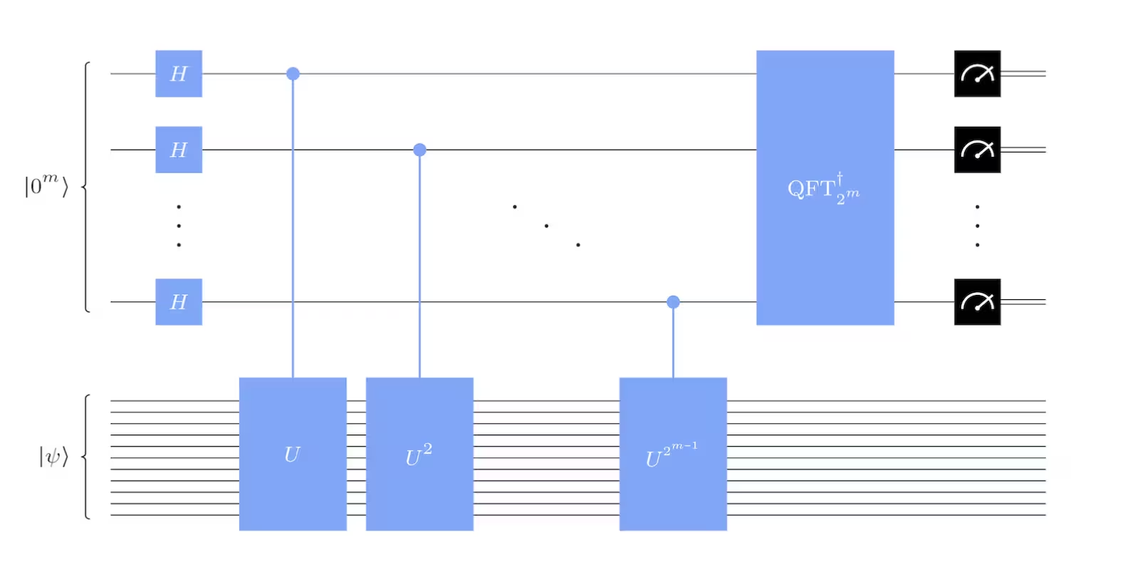
where the number of control qubits (the top $m$ qubits in the figure above) determines the precision of the approximation.

In Shor’s algorithm, we use QPE on the unitary operator $M_a$:

$M_a|y\rangle \equiv |ay \mod N \rangle .$

Here, $|y\rangle$ denotes a computational basis state of the multi-qubit register, where the binary value of the qubits corresponds to the integer $y$. For instance, if $N=15$ and $y = 2$, then $|y\rangle$ is represented by the four-qubit basis state $|0010\rangle$, since four qubits are required to encode numbers up to 15. (If this concept is unfamiliar, see the introductory Qiskit in classrooms module for a refresher on binary encoding of quantum states.)

Now, we need to figure out an eigenstate of this unitary. If we started in the state $|1\rangle$, we can see that each successive application of $U$ will multiply the state of our register by $a \pmod N$, and after $r$ applications we will arrive at the state $|1\rangle$ again. For example with $a = 3$ and $N = 35$:

$$\begin{aligned} M_3|1\rangle &= |3\rangle & \\ M_3^2|1\rangle &= |9\rangle \\ M_3^3|1\rangle &= |27\rangle \\ & \vdots \\ M_3^{(r-1)}|1\rangle &= |12\rangle \\ M_3^r|1\rangle &= |1\rangle \end{aligned}$$

So superpositions of the states in this cycle ($|\psi_j\rangle$) of the form:

$|\psi_j\rangle = \tfrac{1}{\sqrt{r}}\sum_{k=0}^{r-1}{e^{\frac{2 \pi i j k}{r}} |a^k \rangle}$

are all eigenstates of $M_a$. (There are more eigenstates than just these. But we only care about the ones of the form above.)

Check your understanding

Read the question(s) below, think about your answer, then click the triangle to reveal the solution.

Find an eigenstate of the unitary corresponding to $a=2$ and $N = 15$.

Answer:

$$\begin{aligned} M_2|1\rangle &= |2\rangle & \\ M_2^2|1\rangle &= |4\rangle \\ M_2^3|1\rangle &= |8\rangle \\ M_2^4|1\rangle &= |1\rangle \\ \end{aligned}$$

So, the order $r=4$. The eigenstates we're interested in will be an equal superposition of all of the states that were cycled through above, with various phases:

$$\begin{aligned} |\psi_0\rangle &= \frac{1}{2}(|1\rangle+|2\rangle+|4\rangle+|8\rangle) \\ |\psi_1\rangle &= \frac{1}{2}(e^{2 \pi i \frac{0}{4}}|1\rangle+e^{2 \pi i \frac{1}{4}}|2\rangle+e^{2 \pi i \frac{2}{4}}|4\rangle+e^{2 \pi i \frac{3}{4}}|8\rangle) \\ &= \frac{1}{2}(|1\rangle+i|2\rangle-|4\rangle-i|8\rangle) \\ |\psi_2\rangle &= \frac{1}{2}(e^{2 \pi i \frac{0}{4}}|1\rangle+e^{2 \pi i \frac{2}{4}}|2\rangle+e^{2 \pi i \frac{4}{4}}|4\rangle+e^{2 \pi i \frac{6}{4}}|8\rangle) \\ &= \frac{1}{2}(|1\rangle-|2\rangle+|4\rangle-|8\rangle) \\ |\psi_3\rangle &= \frac{1}{2}(e^{2 \pi i \frac{0}{4}}|1\rangle+e^{2 \pi i \frac{3}{4}}|2\rangle+e^{2 \pi i \frac{6}{4}}|4\rangle+e^{2 \pi i \frac{9}{4}}|8\rangle) \\ &= \frac{1}{2}(|1\rangle-i|2\rangle-|4\rangle+i|8\rangle) \\ \end{aligned}$$

Let's say we were able to initialize our qubit state into one of these eigenstates (spoiler — we're not. Or, at least not easily. We'll explain why and what we can do instead shortly). Then we could use QPE to estimate the corresponding eigenvalue, $\omega_j = e^{2 \pi i \theta_j}$ where $\theta_j = \frac{j}{r}$. Then, we'll be able to determine the order $r$ by the simple equation:

$r = \frac{j}{\theta_j}.$

But remember, I said that QPE estimates $\theta_j$ — it doesn't give us an exact value. We need the estimate to be good enough to differentiate between $r$ and $r+1$. The more control qubits $m$, we have, the better the estimate will be. In the problems at the end of the lesson, you'll be asked to determine the minimum $m$ needed to factor a number $N$.

Now, we have to reconcile a problem. All of the above explanation of how to find $r$ begins with preparing the eigenstate $|\psi_j\rangle = \tfrac{1}{\sqrt{r}}\sum_{k=0}^{r-1}{e^{\frac{2 \pi i j k}{r}} |a^k \rangle}$. But we don't know how to do that without already knowing what $r$ is. The logic is circular. We need a way to estimate the eigenvalue without initializing the eigenstate.

Instead of starting with an eigenstate of $M_a$, we can prepare the initial state into the $n$-qubit state corresponding to $|1\rangle$ in binary (as in, $|000...01\rangle$). Although this state itself is obviously not an eigenstate of $M_a$, it is a superposition over all of the eigenstates $|\psi_k\rangle$:

$|1\rangle = \frac{1}{\sqrt{r}} \sum\limits_{k=0}^{r-1}{|\psi_k\rangle}$

Check your understanding

Read the question(s) below, think about your answer, then click the triangle to reveal the solution.

Verify that $|1\rangle$ is equivalent to the superposition over the eigenstates you found for $N=15$ and $a=2$ in the previous check-in question.

Answer:

The four eigenstates were:

$$\begin{aligned} |\psi_0\rangle &= \frac{1}{2}(|1\rangle+|2\rangle+|4\rangle+|8\rangle) \\ |\psi_1\rangle &= \frac{1}{2}(|1\rangle+i|2\rangle-|4\rangle-i|8\rangle) \\ |\psi_2\rangle &= \frac{1}{2}(|1\rangle-|2\rangle+|4\rangle-|8\rangle) \\ |\psi_3\rangle &= \frac{1}{2}(|1\rangle-i|2\rangle-|4\rangle+i|8\rangle) \\ \end{aligned}$$

So,

$$\begin{aligned} \frac{1}{\sqrt{r}} \sum\limits_{k=0}^{r-1}{|\psi_k\rangle} &= \frac{1}{2}(|\psi_0\rangle + |\psi_1\rangle + |\psi_2\rangle + |\psi_3\rangle ) \\ &= \frac{1}{4}(|1\rangle+|2\rangle+|4\rangle+|8\rangle+|1\rangle+i|2\rangle-|4\rangle-i|8\rangle+|1\rangle-|2\rangle+|4\rangle-|8\rangle + |1\rangle-i|2\rangle-|4\rangle+i|8\rangle) \\ &= \frac{1}{4}(4|1\rangle) = |1\rangle \end{aligned}$$

How does this let us find the order $r$? Since the starting state is a superposition over all of the eigenstates of the form listed above, then the QPE algorithm simultaneously estimates each of the $\theta_k$ corresponding to these eigenstates. So, the measurement of the $m$ control qubits at the end will yield an approximation to the value $k/r$ where $k \in \{0,1,2,...,r-1\}$ is one of the eigenvalues randomly chosen. If we repeat this circuit a few times and get a few samples with different values of $k$, we will quickly be able to deduce $r$.

Implement in Qiskit

As we mentioned earlier, our hardware isn't at the point where we can factor huge numbers like RSA1024. We'll just factor a small number to demonstrate how the algorithm works. For this demo, we will use a simplified version of the code presented in the Shor's algorithm tutorial. If you want more details, please visit the tutorial.

We'll run the algorithm using our standard framework for solving quantum problems, called the Qiskit patterns framework. This consists of four steps:

1. Mapping your problem to a quantum circuit
2. Optimize the circuit to be run on quantum hardware
3. Execute your circuit on the quantum computer
4. Post-process the measurements

1. Map

Let's factor $N=15$, selecting $a=2$ to be our co-prime integer.

First, we need to construct the circuit that will implement the modular multiplication unitary, $M_a$. This is actually the trickiest part of the whole implementation, and can be very computationally expensive, depending on how it's done. For this, we'll cheat a little bit: We know that we're starting in the state $|1\rangle$, and from an earlier check-in question,

$$\begin{aligned} M_2|1\rangle &= |2\rangle & \\ M_2|2\rangle &= |4\rangle \\ M_2|4\rangle &= |8\rangle \\ M_2|8\rangle &= |1\rangle \\ \end{aligned}$$

So, we will construct a unitary that does the correct operations on these four states, but leaves all other states alone. This is cheating because we're using our knowledge of the order of $2\bmod 15$ to simplify the unitary. If we were actually trying to factor a number whose factors were unknown to us, we wouldn't be able to do this.

Check your understanding

Read the question(s) below, think about your answer, then click the triangle to reveal the solution.

With your knowledge of how the $M_2$ operator transforms the states above, construct the operator from a series of SWAP gates, which exchange the states of two qubits. (Hint: writing each state $|i\rangle$ in binary will help.)

Answer:

Let's rewrite the action of $M_2$ on the states in binary:

$$\begin{aligned} M_2|0001\rangle &= |0010\rangle \\ M_2|0010\rangle &= |0100\rangle \\ M_2|0100\rangle &= |1000\rangle \\ M_2|1000\rangle &= |0001\rangle \\ \end{aligned}$$

Each of these actions can be accomplished with a simple SWAP. $M_2|0001\rangle$ is achieved by swapping the states of qubit $0$ and $1$. $M_2|0010\rangle$ is achieved by swapping the states of qubit $1$ and $2$. And so on. So, we can deconstruct the $M_2$ matrix into the following series of SWAP gates:

$$M_2 = SWAP(0,1)SWAP(1,2)SWAP(2,3)$$

Remembering that operators act right to left, let's check that this has the effect that we want on each of the states:

$$\begin{aligned} M_2|0001\rangle &= SWAP(0,1)SWAP(1,2)SWAP(2,3)|0001\rangle \\ &= SWAP(0,1)SWAP(1,2)|0001\rangle \\ &= SWAP(0,1)|0001\rangle \\ &=|0010\rangle \checkmark \\ M_2|0010\rangle &= SWAP(0,1)SWAP(1,2)SWAP(2,3)|0010\rangle \\ &= SWAP(0,1)SWAP(1,2)|0010\rangle \\ &= SWAP(0,1)|0100\rangle \\ &=|0100\rangle \checkmark \\ M_2|0100\rangle &= SWAP(0,1)SWAP(1,2)SWAP(2,3)|0100\rangle \\ &= SWAP(0,1)SWAP(1,2)|1000\rangle \\ &= SWAP(0,1)|1000\rangle \\ &=|1000\rangle \checkmark \\ M_2|1000\rangle &= SWAP(0,1)SWAP(1,2)SWAP(2,3)|1000\rangle \\ &= SWAP(0,1)SWAP(1,2)|0100\rangle \\ &= SWAP(0,1)|0010\rangle \\ &=|0001\rangle \checkmark \\ \end{aligned}$$

We can now code the circuit that is equivalent to this operator in Qiskit.

First, we import the necessary packages:

# Import necessary packages

import numpy as np
from fractions import Fraction
from math import floor, gcd, log

from qiskit import QuantumCircuit, QuantumRegister, ClassicalRegister
from qiskit.circuit.library import QFTGate
from qiskit.transpiler import generate_preset_pass_manager
from qiskit.visualization import plot_histogram

from qiskit_ibm_runtime import QiskitRuntimeService
from qiskit_ibm_runtime import SamplerV2 as Sampler

Then, we make the $M_2$ operator:

def M2mod15():
    """
    M2 (mod 15)
    """
    b = 2
    U = QuantumCircuit(4)

    U.swap(2, 3)
    U.swap(1, 2)
    U.swap(0, 1)

    U = U.to_gate()
    U.name = f"M_{b}"

    return U

# Get the M2 operator
M2 = M2mod15()

# Add it to a circuit and plot
circ = QuantumCircuit(4)
circ.compose(M2, inplace=True)
circ.decompose(reps=2).draw(output="mpl", fold=-1)

The QPE algorithm uses a controlled-$U$ gate. So, now that we have an $M_2$ circuit, we need to make it a controlled-$M_2$ circuit:

def controlled_M2mod15():
    """
    Controlled M2 (mod 15)
    """
    b = 2
    U = QuantumCircuit(4)

    U.swap(2, 3)
    U.swap(1, 2)
    U.swap(0, 1)

    U = U.to_gate()
    U.name = f"M_{b}"
    c_U = U.control()

    return c_U

# Get the controlled-M2 operator
controlled_M2 = controlled_M2mod15()

# Add it to a circuit and plot
circ = QuantumCircuit(5)
circ.compose(controlled_M2, inplace=True)
circ.decompose(reps=1).draw(output="mpl", fold=-1)

Now we have our controlled-$U$ gate. But in order to run the Quantum Phase Estimation algorithm, we'll need controlled-$U^2$, controlled-$U^4$, up to controlled-$U^{2^{m-1}}$, where $m$ is the number of qubits used to estimate the phase. The more qubits, the more precise the phase estimation will be. We'll use $m=8$ control qubits for our phase estimation procedure. So, we need:

$$M_{a^{2^k}}|y\rangle \equiv |a^{2^k} y \bmod N \rangle$$

where the index $k$, with $0 \le k \le m-1 = 7$, corresponds to the control qubit. Now let's calculate $a^{2^k}\bmod N$ for each value of $k$:

def a2kmodN(a, k, N):
    """Compute a^{2^k} (mod N) by repeated squaring"""
    for _ in range(k):
        a = int(np.mod(a**2, N))
    return a

k_list = range(8)
b_list = [a2kmodN(2, k, 15) for k in k_list]

print(b_list)

[2, 4, 1, 1, 1, 1, 1, 1]

Since $a^{2^k} \bmod N = 1$ for $k \ge 2$, all of the corresponding operators ($M_8$ and up) are equivalent to the identity. So, we only need to construct one more matrix, $M_4.$

Note: This simplification only works here because the order of $2 \bmod 15$ is $4$. Once $k=2$ (so $2^k = 4$), every subsequent power of the operator is the identity. In general, for larger numbers $N$ or different choices of $a$, you cannot skip constructing the higher powers. This is one reason why this is considered a toy example: the small numbers allow shortcuts that wouldn’t work for larger cases.

def M4mod15():
    """
    M4 (mod 15)
    """
    b = 4
    U = QuantumCircuit(4)

    U.swap(1, 3)
    U.swap(0, 2)

    U = U.to_gate()
    U.name = f"M_{b}"

    return U

# Get the M4 operator
M4 = M4mod15()

# Add it to a circuit and plot
circ = QuantumCircuit(4)
circ.compose(M4, inplace=True)
circ.decompose(reps=2).draw(output="mpl", fold=-1)

And as before, we make it a controlled-$M_4$ operator:

def controlled_M4mod15():
    """
    Controlled M4 (mod 15)
    """
    b = 4
    U = QuantumCircuit(4)

    U.swap(1, 3)
    U.swap(0, 2)

    U = U.to_gate()
    U.name = f"M_{b}"
    c_U = U.control()

    return c_U

# Get the controlled-M4 operator
controlled_M4 = controlled_M4mod15()

# Add it to a circuit and plot
circ = QuantumCircuit(5)
circ.compose(controlled_M4, inplace=True)
circ.decompose(reps=1).draw(output="mpl", fold=-1)

Now, we can put it all together to find the order of $2\bmod 15$ with a quantum circuit, using phase estimation:

# Order finding problem for N = 15 with a = 2
N = 15
a = 2

# Number of qubits
num_target = floor(log(N - 1, 2)) + 1  # for modular exponentiation operators
num_control = 2 * num_target  # for enough precision of estimation

# List of M_b operators in order
k_list = range(num_control)
b_list = [a2kmodN(2, k, 15) for k in k_list]

# Initialize the circuit
control = QuantumRegister(num_control, name="C")
target = QuantumRegister(num_target, name="T")
output = ClassicalRegister(num_control, name="out")
circuit = QuantumCircuit(control, target, output)

# Initialize the target register to the state |1>
circuit.x(num_control)

# Add the Hadamard gates and controlled versions of the
# multiplication gates
for k, qubit in enumerate(control):
    circuit.h(k)
    b = b_list[k]
    if b == 2:
        circuit.compose(
            M2mod15().control(), qubits=[qubit] + list(target), inplace=True
        )
    elif b == 4:
        circuit.compose(
            M4mod15().control(), qubits=[qubit] + list(target), inplace=True
        )
    else:
        continue  # M1 is the identity operator

# Apply the inverse QFT to the control register
circuit.compose(QFTGate(num_control).inverse(), qubits=control, inplace=True)

# Measure the control register
circuit.measure(control, output)

circuit.draw("mpl", fold=-1)

2. Optimize

Now that we've mapped our circuit, the next step is to optimize it to be run on a particular quantum computer. First we need to load the backend.

service = QiskitRuntimeService()

backend = service.backend("ibm_marrakesh")

If you don't have time available on your account or want to use a simulator for any reason, you can run the cell below to set up a simulator that will mimic the quantum device we selected above:

pm = generate_preset_pass_manager(optimization_level=2, backend=backend)

transpiled_circuit = pm.run(circuit)

print(f"2q-depth: {transpiled_circuit.depth(lambda x: x.operation.num_qubits==2)}")
print(f"2q-size: {transpiled_circuit.size(lambda x: x.operation.num_qubits==2)}")
print(f"Operator counts: {transpiled_circuit.count_ops()}")
transpiled_circuit.draw(output="mpl", fold=-1, style="clifford", idle_wires=False)

2q-depth: 188
2q-size: 281
Operator counts: OrderedDict({'sx': 548, 'rz': 380, 'cz': 281, 'measure': 8, 'x': 6})

3. Execute

# Sampler primitive to obtain the probability distribution
sampler = Sampler(backend)

# Turn on dynamical decoupling with sequence XpXm
sampler.options.dynamical_decoupling.enable = True
sampler.options.dynamical_decoupling.sequence_type = "XpXm"
# Enable gate twirling
sampler.options.twirling.enable_gates = True

pub = transpiled_circuit
job = sampler.run([pub], shots=1024)

result = job.result()[0]
counts = result.data["out"].get_counts()

plot_histogram(counts, figsize=(35, 5))

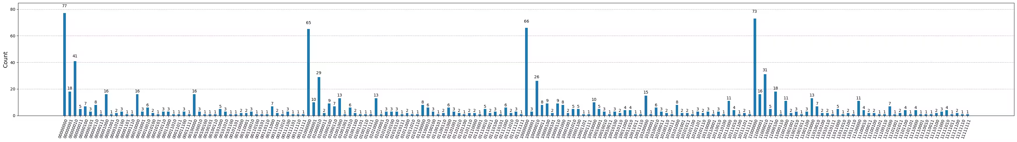
We see four clear peaks at 00000000, 01000000, 10000000, and 11000000, with some counts in other bitstrings due to noise in the quantum computer. We'll ignore these and keep only the dominant four by imposing a threshold: only counts above this threshold are considered a true signal above the noise.

# Dictionary of bitstrings and their counts to keep
counts_keep = {}
# Threshold to filter
threshold = np.max(list(counts.values())) / 2

for key, value in counts.items():
    if value > threshold:
        counts_keep[key] = value

print(counts_keep)

4. Post-process

For Shor's algorithm, quite a lot of the algorithm is performed classically. So, we'll put the rest of it in the "post-processing" step, after we've gotten our measurements from the quantum computer. Each of the measurements above can be converted into integers, which, after we divide by $2^m$, are our approximations for $\frac{k}{r}$, where $k$ is random each time.

a = 2
N = 15

FACTOR_FOUND = False
num_attempt = 0

while not FACTOR_FOUND:
    print(f"\nATTEMPT {num_attempt}:")
    # Here, we get the bitstring by iterating over outcomes
    # of a previous hardware run with multiple shots.
    # Instead, we can also perform a single-shot measurement
    # here in the loop.
    bitstring = list(counts_keep.keys())[num_attempt]
    num_attempt += 1
    # Find the phase from measurement
    decimal = int(bitstring, 2)
    phase = decimal / (2**num_control)  # phase = k / r
    print(f"Phase: theta = {phase}")

    # Guess the order from phase
    frac = Fraction(phase).limit_denominator(N)
    r = frac.denominator  # order = r
    print(f"Order of {a} modulo {N} estimated as: r = {r}")

    if phase != 0:
        # Guesses for factors are gcd(a^{r / 2} ± 1, 15)
        if r % 2 == 0:
            x = pow(a, r // 2, N) - 1
            d = gcd(x, N)
            if d > 1:
                FACTOR_FOUND = True
                print(f"*** Non-trivial factor found: {x} ***")

ATTEMPT 0:
Phase: theta = 0.0
Order of 2 modulo 15 estimated as: r = 1

ATTEMPT 1:
Phase: theta = 0.75
Order of 2 modulo 15 estimated as: r = 4
*** Non-trivial factor found: 3 ***

Conclusion

After going through the module, you may be struck with a new appreciation of the brilliance of Peter Shor to have come up with such a clever algorithm. But hopefully you've also reached a new level of understanding of its deceptive simplicity. Although the algorithm may seem impressively (or intimidatingly) complex, if you break it down into each step of logic and go through it slowly, you, too, will be able to run Shor's algorithm.

While we're far from using this algorithm to factor numbers like RSA1024, our quantum computers are getting better every day, and once a threshold called fault tolerance is reached, then algorithms such as these will be soon to follow. It's an exciting time to be learning about quantum computing!

Problems

Critical concepts:

• Modern cryptographic systems rely on the classical difficulty of factoring large integers.
• Modular arithmetic — including the structures $\mathbb{Z}_N$ and $\mathbb{Z}_N^*$ — provides the mathematical foundation for Shor’s algorithm.
• The problem of factoring an integer $N$ can be reduced to the problem of finding the order of a number modulo $N$.
• Quantum order finding uses quantum phase estimation techniques to determine the period of the function $a^x \mod N$.
• Shor’s algorithm consists of a classical–quantum hybrid workflow that selects a base, performs quantum order finding, and then classically computes the factors from the result.

True/False:

1. T/F The efficiency of Shor's algorithm threatens the security of RSA encryption.
2. T/F Shor's algorithm can be executed efficiently on any modern-day quantum computer.
3. T/F Shor’s algorithm uses quantum phase estimation (QPE) as a key subroutine.
4. T/F The classical part of Shor’s algorithm involves calculating the greatest common divisor (GCD).
5. T/F Shor’s algorithm only works for factoring even numbers.
6. T/F A successful run of Shor’s algorithm always guarantees the correct factors.

Short answer:

1. Why is Shor’s algorithm considered a potential future threat to RSA encryption?
2. Why is finding the period, or order, of a modular exponential function helpful for factoring a number in Shor’s algorithm?

Challenge problems:

1. How many control qubits $m$ do we need for a given number $N$ that we're trying to factor to obtain the precision in the QPE needed to find the correct value of the order $r$?

2. Following the procedure we outlined here to factor 15, now try to factor 21.