Qiskit implementation

In this lesson, we implement some of the ideas from the lesson on entanglement in action, using Qiskit.

# Added by doQumentation — required packages for this notebook
!pip install -q qiskit qiskit-aer

from qiskit import __version__

print(__version__)

2.1.1

from qiskit import QuantumCircuit, QuantumRegister, ClassicalRegister
from qiskit_aer import AerSimulator
from qiskit.visualization import plot_histogram, array_to_latex
from qiskit.result import marginal_distribution
from qiskit.circuit.library import UGate
from math import pi
import random

Here is a quantum circuit implementation of the teleportation protocol.

qubit = QuantumRegister(1, "Q")
ebit0 = QuantumRegister(1, "A")
ebit1 = QuantumRegister(1, "B")
a = ClassicalRegister(1, "a")
b = ClassicalRegister(1, "b")

protocol = QuantumCircuit(qubit, ebit0, ebit1, a, b)

# Prepare ebit used for teleportation
protocol.h(ebit0)
protocol.cx(ebit0, ebit1)
protocol.barrier()

# Alice's operations
protocol.cx(qubit, ebit0)
protocol.h(qubit)
protocol.barrier()

# Alice measures and sends classical bits to Bob
protocol.measure(ebit0, a)
protocol.measure(qubit, b)
protocol.barrier()

# Bob uses the classical bits to conditionally apply gates
with protocol.if_test((a, 1)):
    protocol.x(ebit1)
with protocol.if_test((b, 1)):
    protocol.z(ebit1)

display(protocol.draw(output="mpl"))

The circuit makes use of a few features of Qiskit that we've not yet seen in previous lessons, including the barrier and if_test functions. The barrier function creates a visual separation making the circuit diagram more readable, and it also prevents Qiskit from performing various simplifications and optimizations across the barrier during compilation when circuits are run on real hardware. The if_test function applies an operation conditionally depending on a classical bit or register.

The circuit first initializes $(\mathsf{A},\mathsf{B})$ to be in a $\vert \phi^+\rangle$ state (which is not part of the protocol itself), followed by Alice's operations, then her measurements, and finally Bob's operations. To test that the protocol works correctly, we'll apply a randomly generated single-qubit gate to the initialized $\vert 0\rangle$ state of $\mathsf{Q}$ to obtain a random quantum state vector to be teleported. By applying the inverse (as in, the conjugate transpose) of that gate to $\mathsf{B}$ after the protocol is run, we can verify that the state was teleported by measuring to see that it has returned to the $\vert 0\rangle$ state.

First we'll randomly choose a unitary qubit gate.

random_gate = UGate(
    theta=random.random() * 2 * pi,
    phi=random.random() * 2 * pi,
    lam=random.random() * 2 * pi,
)

display(array_to_latex(random_gate.to_matrix()))

$$\begin{bmatrix} 0.9897212158 & -0.0195080103 - 0.141673401 i \\ 0.0603319186 + 0.1296609988 i & -0.8319925233 + 0.5360378028 i \\ \end{bmatrix}$$

Now we'll create a new testing circuit that first applies our random gate to $\mathsf{Q},$ then runs the teleportation circuit, and finally applies the inverse of our random gate to the qubit $\mathsf{B}$ and measures. The outcome should be $0$ with certainty.

# Create a new circuit including the same bits and qubits used in the
# teleportation protocol.

test = QuantumCircuit(qubit, ebit0, ebit1, a, b)

# Start with the randomly selected gate on Q

test.append(random_gate, qubit)
test.barrier()

# Append the entire teleportation protocol from above.

test = test.compose(protocol)
test.barrier()

# Finally, apply the inverse of the random unitary to B and measure.

test.append(random_gate.inverse(), ebit1)
result = ClassicalRegister(1, "Result")
test.add_register(result)
test.measure(ebit1, result)

display(test.draw(output="mpl"))

Finally, let's run the Aer simulator on this circuit and plot a histogram of the outputs. We'll see the statistics for all three classical bits: the bottom/leftmost bit should always be $0,$ indicating that the qubit $\mathsf{Q}$ was successfully teleported into $\mathsf{B},$ while the other two bits should be roughly uniform.

result = AerSimulator().run(test).result()
statistics = result.get_counts()
display(plot_histogram(statistics))

We can also filter the statistics to focus solely on the test result qubit if we wish, like this:

filtered_statistics = marginal_distribution(statistics, [2])
display(plot_histogram(filtered_statistics))

Superdense coding

Superdense coding is a protocol that, in some sense, achieves a complementary aim to teleportation. Rather than allowing for the transmission of one qubit using two classical bits of communication (at the cost of one e-bit of entanglement), it allows for the transmission of two classical bits using one qubit of quantum communication (again, at the cost of one e-bit of entanglement).

In greater detail, we have a sender (Alice) and a receiver (Bob) that share one e-bit of entanglement. According to the conventions in place for the lesson, this means that Alice holds a qubit $\mathsf{A},$ Bob holds a qubit $\mathsf{B},$ and together the pair $(\mathsf{A},\mathsf{B})$ is in the state $\vert\phi^+\rangle.$ Alice wishes to transmit two classical bits to Bob, which we'll denote by $c$ and $d,$ and she will accomplish this by sending him one qubit.

It is reasonable to view this feat as being less interesting than the one that teleportation accomplishes. Sending qubits is likely to be so much more difficult than sending classical bits for the foreseeable future that trading one qubit of quantum communication for two bits of classical communication, at the cost of an e-bit no less, hardly seems worth it. However, this does not imply that superdense coding is not interesting, for it most certainly is.

Fitting the theme of the lesson, one reason why superdense coding is interesting is that it demonstrates a concrete and (in the context of information theory) rather striking use of entanglement. A famous theorem in quantum information theory, known as Holevo's theorem, implies that without the use of a shared entangled state, it is impossible to communicate more than one bit of classical information by sending a single qubit. (Holevo's theorem is more general than this. Its precise statement is technical and requires explanation, but this is one consequence of it.) So, through superdense coding, shared entanglement effectively allows for the doubling of the classical information-carrying capacity of sending qubits.

Protocol

The following quantum circuit diagram describes the superdense coding protocol:

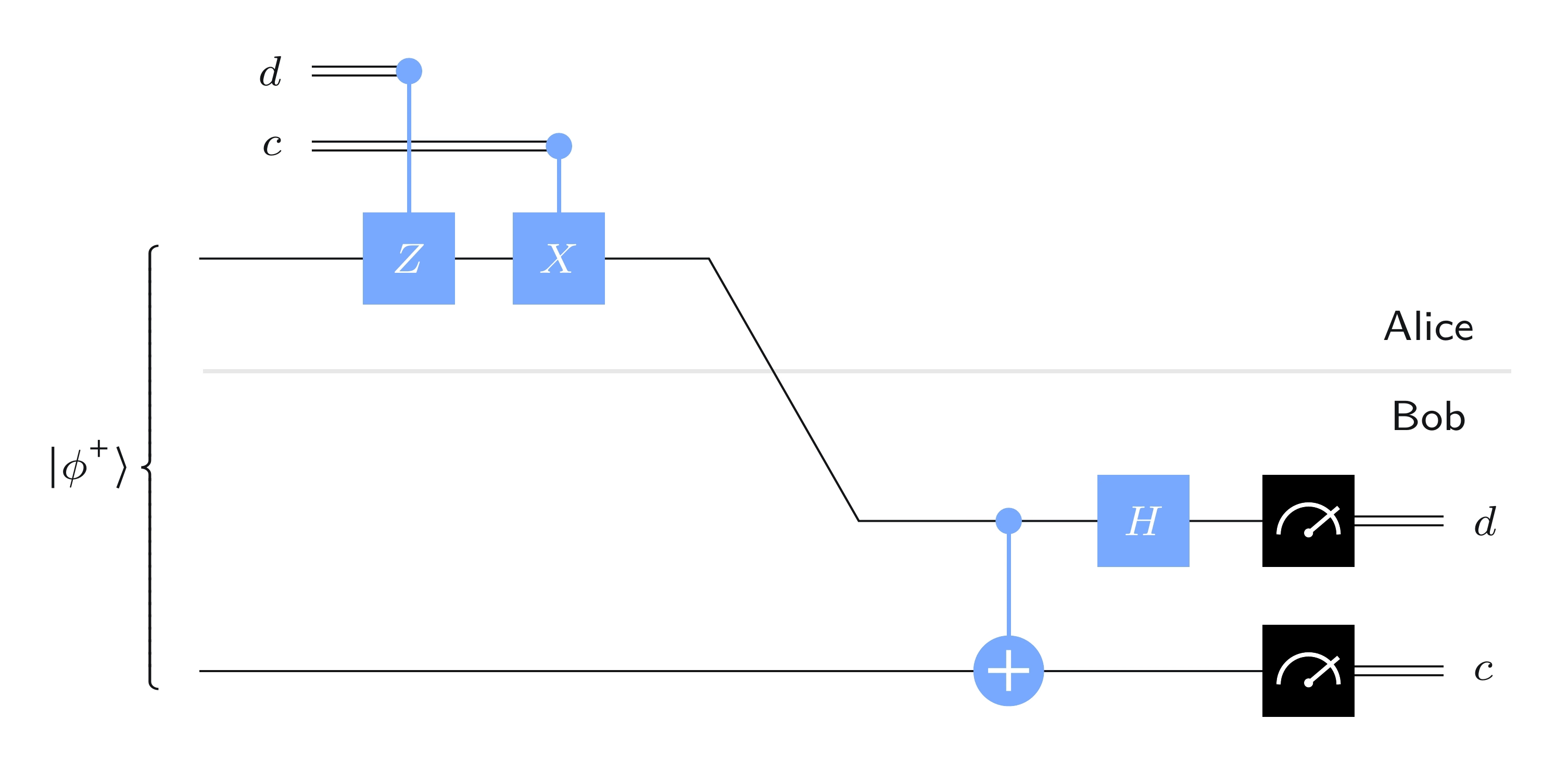
In words, here is what Alice does:

1. If $d=1,$ Alice performs a $Z$ gate on her qubit $\mathsf{A}$ (and if $d=0$ she does not).

2. If $c=1,$ Alice performs an $X$ gate on her qubit $\mathsf{A}$ (and if $c=0$ she does not).

Alice then sends her qubit $\mathsf{A}$ to Bob.

What Bob does when he receives the qubit $\mathsf{A}$ is to first perform a controlled-NOT gate, with $\mathsf{A}$ being the control and $\mathsf{B}$ being the target, and then he applies a Hadamard gate to $\mathsf{A}.$ He then measures $\mathsf{B}$ to obtain $c$ and $\mathsf{A}$ to obtain $d,$ with standard basis measurements in both cases.

Analysis

The idea behind this protocol is simple: Alice effectively chooses which Bell state she would like to be sharing with Bob, she sends Bob her qubit, and Bob measures to determine which Bell state Alice chose.

That is, they initially share $\vert\phi^+\rangle,$ and depending upon the bits $c$ and $d,$ Alice either leaves this state alone or shifts it to one of the other Bell states by applying $\mathbb{I},$ $X,$ $Z,$ or $XZ$ to her qubit $\mathsf{A}.$

$$\begin{aligned} (\mathbb{I} \otimes \mathbb{I}) \vert \phi^+ \rangle & = \vert \phi^+\rangle \\ (\mathbb{I} \otimes Z) \vert \phi^+ \rangle & = \vert \phi^-\rangle \\ (\mathbb{I} \otimes X) \vert \phi^+ \rangle & = \vert \psi^+\rangle \\ (\mathbb{I} \otimes XZ) \vert \phi^+ \rangle & = \vert \psi^-\rangle \end{aligned}$$

Bob's actions have the following effects on the four Bell states:

$$\begin{aligned} \vert \phi^+\rangle & \mapsto \vert 00\rangle\\ \vert \phi^-\rangle & \mapsto \vert 01\rangle\\ \vert \psi^+\rangle & \mapsto \vert 10\rangle\\ \vert \psi^-\rangle & \mapsto -\vert 11\rangle\\ \end{aligned}$$

This can be checked directly, by computing the results of Bob's operations on these states one at a time.

So, when Bob performs his measurements, he is able to determine which Bell state Alice chose. To verify that the protocol works correctly is a matter of checking each case:

• If $cd = 00,$ then the state of $(\mathsf{B},\mathsf{A})$ when Bob receives $\mathsf{A}$ is $\vert \phi^+\rangle.$ He transforms this state into $\vert 00\rangle$ and obtains $cd = 00.$

• If $cd = 01,$ then the state of $(\mathsf{B},\mathsf{A})$ when Bob receives $\mathsf{A}$ is $\vert \phi^-\rangle.$ He transforms this state into $\vert 01\rangle$ and obtains $cd = 01.$

• If $cd = 10,$ then the state of $(\mathsf{B},\mathsf{A})$ when Bob receives $\mathsf{A}$ is $\vert \psi^+\rangle.$ He transforms this state into $\vert 10\rangle$ and obtains $cd = 10.$

• If $cd = 11,$ then the state of $(\mathsf{B},\mathsf{A})$ when Bob receives $\mathsf{A}$ is $\vert \psi^-\rangle.$ He transforms this state into $-\vert 11\rangle$ and obtains $cd = 11.$ (The negative-one phase factor has no effect here.)

Superdense coding implementation

Here is a simple implementation of superdense coding where we specify the circuit itself depending on the bits to be transmitted. First we'll choose two bits to be transmitted. (Later we'll choose them randomly, but for now we'll just make an arbitrary choice.)

c = "1"
d = "0"

Now we'll build the circuit accordingly. Here we'll allow Qiskit to use the default names for the qubits: $\mathsf{q}_0$ for the top qubit and $\mathsf{q}_1$ for the bottom one.

protocol = QuantumCircuit(2)

# Prepare ebit used for superdense coding
protocol.h(0)
protocol.cx(0, 1)
protocol.barrier()

# Alice's operations
if d == "1":
    protocol.z(0)
if c == "1":
    protocol.x(0)
protocol.barrier()

# Bob's actions
protocol.cx(0, 1)
protocol.h(0)
protocol.measure_all()

display(protocol.draw(output="mpl"))

Not much is new here, except the measure_all function, which measures all of the qubits and puts the results into a single classical register (and therefore having two bits in this case).

Running the Aer simulator produces the expected output.

result = AerSimulator().run(protocol).result()
statistics = result.get_counts()

for outcome, frequency in statistics.items():
    print(f"Measured {outcome} with frequency {frequency}")

display(plot_histogram(statistics))

Measured 10 with frequency 1024

Now let's use an additional qubit as a random bit generator — essentially to flip fair coins. We'll use it to randomly choose $c$ and $d,$ and then run the superdense coding protocol.

rbg = QuantumRegister(1, "coin")
ebit0 = QuantumRegister(1, "A")
ebit1 = QuantumRegister(1, "B")

Alice_c = ClassicalRegister(1, "Alice c")
Alice_d = ClassicalRegister(1, "Alice d")

test = QuantumCircuit(rbg, ebit0, ebit1, Alice_d, Alice_c)

# Initialize the ebit
test.h(ebit0)
test.cx(ebit0, ebit1)
test.barrier()

# Use the 'coin' qubit twice to generate Alice's bits c and d.
test.h(rbg)
test.measure(rbg, Alice_c)
test.h(rbg)
test.measure(rbg, Alice_d)
test.barrier()

# Now the protocol runs, starting with Alice's actions, which depend
# on her bits.
with test.if_test((Alice_d, 1), label="Z"):
    test.z(ebit0)
with test.if_test((Alice_c, 1), label="X"):
    test.x(ebit0)
test.barrier()

# Bob's actions
test.cx(ebit0, ebit1)
test.h(ebit0)
test.barrier()

Bob_c = ClassicalRegister(1, "Bob c")
Bob_d = ClassicalRegister(1, "Bob d")
test.add_register(Bob_d)
test.add_register(Bob_c)
test.measure(ebit0, Bob_d)
test.measure(ebit1, Bob_c)

display(test.draw(output="mpl"))

Running the Aer simulator shows the results: Alice and Bob's classical bits always agree.

result = AerSimulator().run(test).result()
statistics = result.get_counts()
display(plot_histogram(statistics))

Qiskit implementation

We can implement the CHSH game, together with the quantum strategy defined above, in Qiskit as follows.

First, here's the definition of the game itself, which allows an arbitrary strategy to be plugged in as an argument.

def chsh_game(strategy):
    # This function runs the CHSH game, using the strategy (a function
    # from two bits to two bits), returning 1 for a win and 0 for a loss.

    # Choose x and y randomly
    x, y = random.randint(0, 1), random.randint(0, 1)

    # Use the strategy to determine a and b
    a, b = strategy(x, y)

    # Decide if the strategy wins or loses
    if (a != b) == (x & y):
        return 1  # Win
    return 0  # Lose

Now we'll create a function that outputs a circuit depending on the questions for Alice and Bob. We'll let the qubits have their default names for simplicity, and we'll use the built-in $R_y(\theta)$ gate for Alice and Bob's actions.

def chsh_circuit(x, y):
    # This function creates a `QuantumCircuit` implementing the quantum
    # strategy described above (including the e-bit preparation).

    qc = QuantumCircuit(2, 2)

    # Prepare an e-bit
    qc.h(0)
    qc.cx(0, 1)
    qc.barrier()

    # Alice's actions
    if x == 0:
        qc.ry(0, 0)
    else:
        qc.ry(-pi / 2, 0)
    qc.measure(0, 0)

    # Bob's actions
    if y == 0:
        qc.ry(-pi / 4, 1)
    else:
        qc.ry(pi / 4, 1)
    qc.measure(1, 1)

    return qc

Here are the four possible circuits, depending on which questions are asked.

# Draw the four possible circuits

print("(x,y) = (0,0)")
display(chsh_circuit(0, 0).draw(output="mpl"))

print("(x,y) = (0,1)")
display(chsh_circuit(0, 1).draw(output="mpl"))

print("(x,y) = (1,0)")
display(chsh_circuit(1, 0).draw(output="mpl"))

print("(x,y) = (1,1)")
display(chsh_circuit(1, 1).draw(output="mpl"))

(x,y) = (0,0)

(x,y) = (0,1)

(x,y) = (1,0)

(x,y) = (1,1)

Now we'll create a job using the Aer simulator that runs the circuit a single time for a given input pair $(x,y).$

def quantum_strategy(x, y):
    # This function runs the appropriate quantum circuit defined above
    # one time and returns the measurement results

    # Setting `shots=1` to run the circuit once
    result = AerSimulator().run(chsh_circuit(x, y), shots=1).result()
    statistics = result.get_counts()

    # Determine the output bits and return them
    bits = list(statistics.keys())[0]
    a, b = bits[0], bits[1]
    return a, b

Finally, we'll play the game 1000 times and compute the fraction that the strategy wins.

NUM_GAMES = 1000
TOTAL_SCORE = 0

for _ in range(NUM_GAMES):
    TOTAL_SCORE += chsh_game(quantum_strategy)

print("Fraction of games won:", TOTAL_SCORE / NUM_GAMES)

Fraction of games won: 0.867

We can also define a classical strategy and see how well it works. This is just one strategy — others can be tested by changing the code — but it is among the optimal classical strategies.

def classical_strategy(x, y):
    # This function implements just one example of an optimal classical
    # strategy for the CHSH game. Other classical strategies can be
    # implemented by changing the bit values assigned to a and b.

    # Alice's answer
    if x == 0:
        a = 0
    elif x == 1:
        a = 1

    # Bob's answer
    if y == 0:
        b = 1
    elif y == 1:
        b = 0

    return a, b

Again let's play the game 1000 times to see how well it works.

NUM_GAMES = 1000
TOTAL_SCORE = 0

for _ in range(NUM_GAMES):
    TOTAL_SCORE += chsh_game(classical_strategy)

print("Fraction of games won:", TOTAL_SCORE / NUM_GAMES)

Fraction of games won: 0.747

Although there's randomness involved, the statistics are very unlikely to deviate too much after 1000 runs. The quantum strategy wins about 85% of the time while a classical strategy can't win more than about 75% of the time.